1.6.1: Latitude and Longitude

 The Geographic Coordinate System

Latitude and longitude comprises a grid system of lines encircling the globe and is used to determine the locations of points on the Earth. 

Figure \(\PageIndex{1}\): The Geographic Grid: Latitude and Longitude. (CC0 1.0; Djexplo via Wikimedia Commons).

Figure \(\PageIndex{1}\) shows two globe diagrams placed side by side, each illustrating the coordinate grid used in geography.

On the left globe, the continents of North and South America are visible in yellow, surrounded by blue oceans. A network of curved lines covers the globe, representing latitude (horizontal parallels) and longitude (vertical meridians). A dashed horizontal line runs across the center of this globe, indicating the equator, which divides the Earth into the Northern and Southern Hemispheres.

On the right globe, parts of Europe, Africa, and Asia are shown. The same grid of latitude and longitude lines is visible. A dashed vertical line runs from the top to the bottom of this globe, representing the prime meridian, which divides the Earth into the Eastern and Western Hemispheres.

The two globes together emphasize how the coordinate system is organized:

• Parallels run east–west and measure distance north or south of the equator.
• Meridians run north–south and measure distance east or west of the prime meridian.

Lines of latitude also called parallels, run east to west. Latitude lines always run parallel to each other, and hence, they are always an equal distance apart. Latitude lines never converge or cross. The latitudes are circles with their size reducing from the center to the poles. Parallels of latitude measure distance north or south of the equator.  

Figure \(\PageIndex{2}\): The Equator. (CC BY-SA 4.0; The National Atlas, Courtesy Ritter, Michael E via The Physical Environment).

The equator shown in Figure \(\PageIndex{2}\) is the central most parallel of latitude. The latitude of a particular location is the distance, measured in degrees, between that place and the equator along a meridian, or line of longitude. The equator is 0^o latitude, and the North and South Poles are located at 90^o north and 90^o south latitude respectively. In other words, values for latitude range from a minimum of 0^o to a maximum of 90^o.

If the Earth were a perfect sphere (which it isn't), the distance, or the length, of 1^o of latitude would be constant everywhere. In reality, the Earth is slightly flattened at the poles, so the length of 1^o of latitude at the poles is slightly more than at the equator. At the equator, the length of 1^o of latitude is equal to 110.6 km (68.7 miles) and at the poles, the length of 1^o of latitude is equal to 111.7 km (69.4 miles). For our purposes, we will assume the length of one degree of latitude is 111 km.

Figure \(\PageIndex{3}\): The important parallels of latitude shown in a world map drawn using Robinson Projection. (CC BY-SA 4.0; PJsg1011, via Wikimedia Commons).

The important parallels of latitude are shown in Figure \(\PageIndex{3}\). The image shows a world map with key lines of latitude and longitude highlighted and labeled.

The map is presented in an oval projection with continents outlined in light colors and oceans in pale blue. A grid of faint curved lines covers the map, representing latitude and longitude. Several important horizontal lines of latitude are clearly marked and labeled:

• The Equator (0°) runs across the center of the map in green.
• The Tropic of Cancer (23°26′ N) is shown above the equator in red.
• The Tropic of Capricorn (23°26′ S) is shown below the equator in red.
• The Arctic Circle (66°33′ N) appears near the top in purple.
• The Antarctic Circle (66°33′ S) appears near the bottom in purple.

A vertical line of longitude, the Prime Meridian (0°), is shown in purple running from the North Pole to the South Pole through Europe and Africa.The labeled lines intersect at right angles, forming a geographic grid.

Figure \(\PageIndex{4}\): Longitude (CC BY-SA 4.0; The National Atlas, Courtesy Ritter, Michael E via The Physical Environment)

Figure \(\PageIndex{4}\) shows a circular polar projection map of the world, centered on the North Pole, with a coordinate grid of latitude and longitude.

The map is arranged like a circle, with the North Pole at the center. From the center, lines of longitude radiate outward like spokes on a wheel, labeled with degrees such as 0°, 45°E, 90°E, 135°E, 180°, 135°W, 90°W, and 45°W. These lines divide the map into equal angular sections.

Concentric circular rings represent lines of latitude, moving outward from the pole toward lower latitudes. The outer edge of the circle represents lower latitudes, while the center represents the highest latitude at 90° North.

Lines of longitude, also called meridians, run from north to south. Meridians are farthest apart at the equator, and converge at the North and South Poles. Lines of longitude shown in Figure \(\PageIndex{4}\) measure distance east or west of the prime meridian. The longitude of a particular location is the distance along a parallel, measured in degrees, between that place and the prime meridian. The prime meridian passes through the old Royal Observatory at Greenwich, England, and is sometimes referred to as the Greenwich meridian. Since meridians are farthest apart at the equator and converge at the poles, the distance in kilometers (or miles) of 1^o of longitude varies from a maximum at the equator, to a minimum at the poles. At the equator the approximate length of 1^o is approximately 111 km (69 mi.). At 60^o north and south latitudes, the length of 1^o of longitude is approximately 55.5 km (34.5 miles), or half what it is at the equator.

Figure \(\PageIndex{5}\): The prime meridian. (CC BY-SA 4.0; The National Atlas, Courtesy Ritter, Michael E via The Physical Environment).

The prime meridian highlighted in Figure \(\PageIndex{5}\), which runs through Greenwich, England, is referred to as 0^o longitude. Points are measured east or west of the prime meridian until one reaches the opposite side of the prime meridian, which is referred to as the International Date Line. This is considered 180^o longitude, and is the highest value which longitude can take. In other words, values for longitude range from a minimum of 0^o to a maximum of 180^o. The Prime Meridian along with the 180^o meridian together make a great circle.

An infinite number of parallels or meridians can be drawn on a globe. Thus, parallels and meridians exist for any point on the Earth. Generally, only selected parallels and meridians are marked on maps and globes, and these are usually spaced equal distances apart. Parallels and meridians always intersect each other at right angles. In order to locate a particular point on the Earth, a latitude and a longitude measurement is necessary. As stated above, these measurements are in degrees, but sometimes measurements smaller than degrees are necessary. In this case, minutes and seconds are used.

When we travel, we usually like to take the shortest route between two locations. If you pass a plane through the center of a sphere, the intersection of the plane and the surface of the sphere creates a great circle. Planes passing through any other part of a sphere without going through the center create small circles. An arc of a great circle is the shortest distance between two points on a sphere and therefore is the preferred route for planes traveling great distances, like crossing an ocean. The concept of great and small circles relates to meridians (longitude) and parallels (latitude). Meridians are half of a great circle (180^o) whose ends are at the North and South poles. All meridians along with their opposite meridian form great circles. Most parallels of latitude are small circles, except for the equator which is a great circle.

Figure \(\PageIndex{6}\): Great Circle.
(CC BY-SA 3.0; via Wikimedia Commons ).

 

 

 

Figure \(\PageIndex{7}\): Small Circle.
(CC BY-SA 3.0; via Wikimedia Commons )

Figure \(\PageIndex{6}\) shows a globe covered with a latitude and longitude grid, with a tilted ring-like band wrapping around the Earth. The globe is drawn with many curved lines:

• Horizontal circles (parallels) represent latitude.
• Vertical curved lines (meridians) represent longitude.

Across the middle of the globe, a thick oval-shaped band wraps diagonally around the surface rather than horizontally. This band appears tilted relative to the grid. This tilted band represents the equator as viewed from an angle, or the idea that Earth is a sphere and not flat, so lines like the equator may appear curved or tilted depending on the viewing perspective. The grid lines curve and converge toward the top and bottom of the sphere, showing how longitude lines meet at the poles and how latitude lines form smaller circles toward the poles.

Figure \(\PageIndex{7}\) shows a three-dimensional globe covered with a latitude and longitude grid, along with a tilted circular slice positioned above the surface.

The globe is drawn as a sphere with many curved lines:

• Horizontal circles (parallels) represent lines of latitude.
• Vertical curved lines (meridians) represent lines of longitude that converge toward the poles.

Near the upper right portion of the globe, a separate curved slice appears to be cut from the surface. This slice is angled and slightly lifted away from the globe, revealing part of the spherical surface beneath it. The shape of the slice follows the curvature of the globe, indicating it is a section of a circular band. The slice represents a portion of a small circle or a parallel of latitude, viewed in isolation to help visualize how these circles wrap around the globe.

For more information about other locational systems, read the optional section  "Digging Deeper Into Locational Systems"

Dig Deeper into Locational Systems

United States Public Land Survey (USPLS)

Latitude and longitude gives us an easy way of locating points on the Earth. Instead of a point, we may wish to identify land areas. In the United States, the United States Public Land Survey (USPLS), conceived by Thomas Jefferson, is used to identify parcels of land. The USPLS is actually a means of describing parcels of land, but like latitude and longitude, the USPLS is basically a grid that can be used to identify location.

Figure \(\PageIndex{8}\):bUnited States Public Land Survey Townships and Ranges. (CC BY-SA 4.0 ; Ritter, Michael E via The Physical Environment).

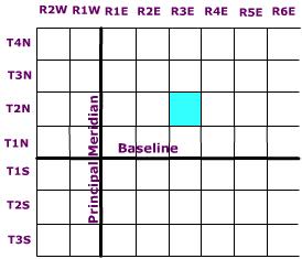
Across the United States, several principal meridians (lines of longitude) have been selected to define "columns" of ranges every six miles either east or west of a particular principal meridian. In a similar fashion, "rows" of townships are delimited every six miles either north or south of a particular baseline, that coincides with a line of latitude. This creates a grid work of townships and ranges encompassing 36 square miles in area. Actually, an individual cell in this grid is sometimes referred to simply as a township.

Figure \(\PageIndex{8}\) shows a rectangular grid organized around two perpendicular reference lines: an east-west Baseline and a north-south Principal Meridian. Key elements:

Township tiers (North-South): Horizontal rows measuring 6 miles north to south, numbered progressively away from the baseline, such as T1N and T2N moving north, or T1S moving south.

Ranges (East-West): Vertical columns measuring 6 miles east to west, numbered progressively away from the principal meridian, such as R1E and R2E moving east, or R1W moving west.

Township cells: The 6-mile by 6-mile area formed where a township tier and a range intersect. Each township cell encompasses 36 square miles.

Figure \(\PageIndex{9}\): United States Public Land Survey Sections. (CC BY-SA 4.0 ; Ritter, Michael E via The Physical Environment).

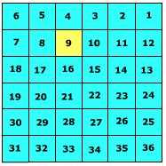
A township is subdivided into 36 one square mile sections. Sections are numbered beginning at the upper right and working left to section 6, then down to 7, and then right across to section 12 ending with 36 sections as shown in Figure \(\PageIndex{9}\). Key elements include: 

Serpentine numbering: The numbers follow a snake-like path. It begins in the northeast corner with Section 1, counts west across the top row to Section 6 in the northwest corner, drops down to Section 7, counts east to Section 12, and alternates back and forth until reaching Section 36 in the southeast corner.

Scale: Each section measures 1 mile on each side, equal to 1 square mile or 640 acres.

Figure \(\PageIndex{10}\): Subdivision of a section.  (CC BY-SA 4.0 ; Ritter, Michael E via The Physical Environment).

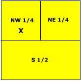
Each section is 640 acres in size and can be further subdivided into smaller units by either halving or quartering the section as shown in Figure \(\PageIndex{10}\) and described according to direction. For instance, the letter X is located in the NW 1/4, S9, T2N, R3E. 

Key elements:

Quarter sections: Dividing the 640-acre square into four 160-acre quadrants: Northwest quarter (NW 1/4), Northeast quarter (NE 1/4), Southwest quarter (SW 1/4), and Southeast quarter (SE 1/4).

Further division: Each 160-acre quarter can be divided again into 40-acre parcels (such as the NW 1/4 of the NW 1/4) or halved into 80-acre parcels.

Reading order: Legal descriptions are written from smallest parcel to largest parent grid, such as NW 1/4, Section 9, T2N, R3E.

All United States Geological Survey topographic maps show the township, range, and section information on them. Figure \(\PageIndex{11}\) is a portion of the Whitewater, WI 1:24000 USGS topographic map. Township and Range information is found printed in red along the bottom and left margins (R 17E, T3N). Section boundaries are printed in red and their number designation is printed in the center of the section.

Figure \(\PageIndex{11}\): USPLS coordinates on topographic map. (CC BY-SA 4.0 ; Ritter, Michael E via The Physical Environment).

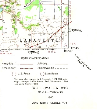
 Figure \(\PageIndex{11}\) shows a portion of a United States Geological Survey (USGS) topographic map, focused on the Whitewater, Wisconsin area.

The map includes:

• A section of terrain with contour lines in brown, indicating changes in elevation.
• Light green areas representing vegetation or forested land, and white or beige areas indicating less vegetated or developed land.
• The place name “LAFAYETTE” appears prominently across the center of the map.

Several coordinate and reference elements are visible:

• Township and Range information is printed in red along the edges, such as T3N (Township 3 North) and R17E (Range 17 East).
• A coordinate value “4735000m N” appears along the right edge, indicating a northing value in the UTM (Universal Transverse Mercator) system.
• A longitude value “88°30′” is also shown along the edge.

At the bottom, there is a road classification legend showing different line styles for road types, including:

• Heavy-duty roads
• Medium-duty roads
• Light-duty roads
• Unimproved dirt roads
• U.S. routes and state routes

Additional text at the bottom includes:

• “WHITEWATER, WIS.”
• Coordinates for the map location: 42°45′ N, 88°30′15″ W
• Map series and reference details

The Universal Transverse Mercator (UTM) Grid

Though a spherical coordinate system like latitude and longitude is convenient for large areas, it is cumbersome for small areas. The need for accurate measurements within small areas was realized with the increasing range of artillery during the First and Second World Wars. This spurred the development of rectangular coordinate grid systems as plane rectangular geometry formulas were simpler than spherical geometry formulas upon which latitude and longitude is derived from. The Universal Transverse Mercator (UTM) Grid is one such system.

The Universal Transverse Mercator Grid shown in Figure \(\PageIndex{12}\), divides the world into 60 north-south zones, each covering a strip 6° wide in longitude between 84N and 80S. Poleward the Universal Stereographic grid (UPS) is used. These longitude zones are numbered (called the "zone number") from Zone 1, between 180° and 174° west longitude, progressing eastward to Zone 60, between 174° and 180° east longitude. Each longitude zone is subdivided into a latitude zone is 8 degrees high north and south of the equator, and lettered starting from "C" at 80° S, increasing up to "X" (called the "zone designator"). The letters "I" and "O" are omitted because of their similarity to the digits one (1) and zero(0). X spans 12° of latitude.

Figure \(\PageIndex{12}\): The UTM Zones The grid reference is read "right, up", and written with the longitude zone first. The example identified by the arrows is "17T". (CC BY-SA 4.0 ; Ritter, Michael E via The Physical Environment)

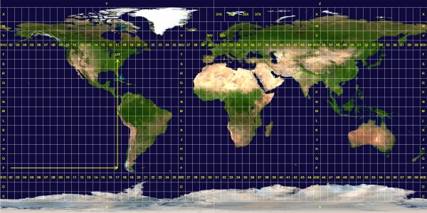
Each longitude zone is subdivided into an eastern and western half by drawing a line down the middle called the "central meridian". A point can be described by its distance east of the origin, called its "easting" value. The central meridian is assigned a false easting of 500,000 meters to insure positive coordinates. Any easting value greater than 500,000 meters indicates a point east of the central meridian. Any easting value less than 500,000 meters indicates a point west of the central meridian. A point's north-south origin depends on the hemisphere it is in. In the northern hemisphere, the origin is the equator and all distances north (or ‘northings’) are measured from the equator. In the southern hemisphere the origin is the south pole and all northings are measured from there. When writing UTM coordinates, the easting is always first and the northing is after it.

Figure \(\PageIndex{13}\): UTM coordinates on topographic map. (CC BY-SA 4.0 ; Ritter, Michael E via The Physical Environment).

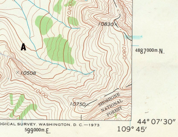
The UTM grid is printed on all U.S. Geological Survey (USGS) maps as blue tick marks in the margins, or as full grid lines. The spacing of the tick marks or grid lines depends on the scale of the map. In Figure \(\PageIndex{13}\) Point A on the topographic map is located at 599000 E., 4887000 N.