1.4.4: Geography and the Scientific Method

Geographic Inquiry 

The steps in geographic inquiry are embodied in the "scientific method". The scientific method consists of systematic observation, formulation, testing and revision of hypotheses. If a hypothesis withstands the scrutiny of repeated experimentation and review it may be elevated to a theory. Theories may undergo revision as new data and research methods are improved.

Figure \(\PageIndex{1}\): The Scientific Method. (CC BY-SA 4.0 , Courtesy Michael E. Ritter via The Physical Environment).

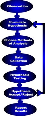
As illustrated in Figure \(\PageIndex{1}\) a vertical flowchart representing the steps of the scientific method.

At the top of the diagram is the first step, labeled “Observation.” Directly below it is “Formulate Hypothesis.” The flow continues downward in a straight line through the steps: “Choose Methods of Analysis,” “Data Collection,” and “Hypothesis Testing.”

After testing, the next step is “Hypothesis Accept/Reject.” From this step, an arrow branches to the right, indicating a decision point. The process then continues downward to the final step, “Report Results.”

All steps are enclosed in oval shapes connected by arrows, showing a clear sequence from top to bottom.

Let's look at a very simple example of how you as a geographer could use the scientific method.

Observation

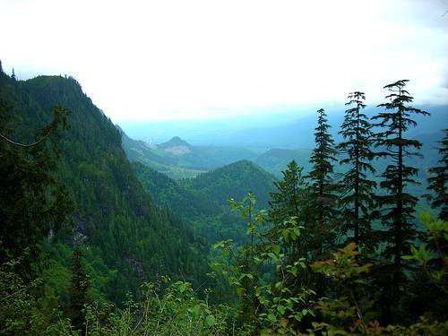
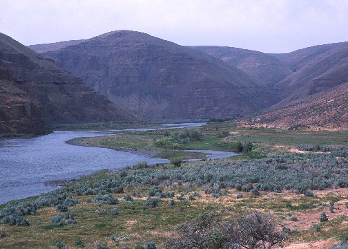
During a trip through the Cascade Range of Oregon you notice that the western slope tends to have more lush vegetation than the eastern slope and wonder why. Our experience tells us that vegetation requires moisture to live, and more lush vegetation is found where precipitation is abundant. Could it be that the western slopes are rainier than the eastern slopes given the spatial variation in vegetation? Figure \(\PageIndex{2}\) and Figure \(\PageIndex{3}\) pictorially reveal the difference between the eastern and western slope of Cascade Range Mountains. 

Figure \(\PageIndex{2}\): View of western slope of Cascade Range mountains. (CC BY 2.0; Christy Gordon via Flickr).

Figure \(\PageIndex{3}\): Near Condon, OR, east slope of Cascade Range. (CC BY-SA 4.0; Michael E. Ritter via The Physical Environment).

Hypothesis formulation

A hypothesis is referred to as "an educated guess". That is, upon recognizing a particular pattern displayed by Earth phenomenon, the geographer offers a "guess" or explanation as to what caused it. Previous research serves as the foundation for constructing hypotheses. Given our initial observation and past experience we suggest that there is a relationship between slope orientation and precipitation.

A hypothesis is stated in a clear and concise way so that it can be tested through data collection and analysis. When constructing a hypothesis, scientists actually formulate two hypotheses related to their problem. The null hypothesis is a statement of no relationship. This is the hypothesis we will either reject or not reject.

• The null hypothesis (Ho) for our problem is:
  • H_o: There is no relationship between slope orientation and precipitation.
• The alternative hypothesis is a statement of relationship. The alternate hypothesis is:
  • H_a: There is a relationship between slope orientation and precipitation.

Determine the methods used to test the hypothesis

There are a variety of quantitative and qualitative methods to test our hypothesis. One could calculate the average precipitation for the western and eastern slopes and apply a difference of means test like t-test. T-test is a statistical test used to see if there is a statistically significant difference between the mean precipitation of the western and eastern slopes. 

Data collection

In order to test our hypothesis we must collect a sample of data. For most cases, a sample set of 30 will suffice. Primary data can be collected in the field and analyzed, or secondary data that has already been published can be used. Precipitation data is available from a variety of public and private sources.

Figure \(\PageIndex{4}\): Precipitation in Oregon. Note linear purple areas of of high precipitation along western slopes of the mountains. This is a map of Oregon's annual average precipitation from 1961 to 1990 where the west gets more rain than the east. (CC BY-SA 4.0, Courtesy Wikimedia Commons).

Figure \(\PageIndex{4}\) is a color-coded map of Oregon showing average annual precipitation from 1961 to 1990. A legend below the map displays precipitation ranges from 5 inches and less to 180.1 to 200 inches.

The map shows a clear regional pattern. Western Oregon, especially along the Pacific coast and mountain ranges, receives the highest precipitation. Eastern Oregon receives much less precipitation overall.

The legend uses warm colors such as red and light orange for the lowest precipitation values and darker greens to purples for the highest precipitation values. Because the colors represent rainfall amounts, the text description is necessary so that the map’s meaning is not conveyed by color alone.

The map also labels major geographic features and neighboring areas, including the Pacific Ocean, the Columbia River, and the states of Washington, Idaho, California, and Nevada.

Analysis: Testing the hypothesis

A geographer often starts their analysis using some way to visualize the spatial pattern of precipitation. A map showing the geographic pattern of precipitation can be created if data from several places have been obtained. Or a graph of precipitation with the y-axis scaled for precipitation and x-axis for distance between locations along a transect. Statistics describing the data are usually calculated. The mean or average of each data set (west side and east side of the mountains) are determined and finally the hypothesis is tested using the difference of means test.

Hypothesis Acceptance/Rejection (Explanation)

After testing our hypothesis we will either accept or reject our null hypothesis. In reality, we can't prove our hypothesis correct, we can only disprove it based on our analysis. That is, we reject the null hypothesis that there is no difference in precipitation based on the data that we have collected. If new data or better data collection techniques are available in the future, they may lead us to conclude that we cannot reject our null hypothesis. Hence it is hard to prove a hypothesis is correct as new information and understanding may present itself in the future.

Report Results

If we can accepted our hypothesis then we can report our results so others can scrutinize our work and test our hypothesis under different circumstances.If our null hypothesis is rejected we can turn to our alternative hypothesis or restate the null hypothesis in a different way. Thus, applying the scientific method can be an iterative process. If our work can be replicated many times under different circumstance the hypothesis can be elevated to a theory. A theory can be a hypothesis or group of hypotheses that has been validated through repeated experiments and coming to the same conclusion.