4.7: Plate Motions on a Sphere

Now that we understand plate motion on a plane, let's move to a sphere. In order to move to a sphere, we need to master five ideas/concepts.

1. Spherical Coordinates
2. Euler Pole
3. Angular Distance
4. Relative motion from Euler Poles
   • Reference Frame
5. Velocity and direction of motion at a point

Spherical Coordinates

Figure \(\PageIndex{1}\): Latitude and Longitude

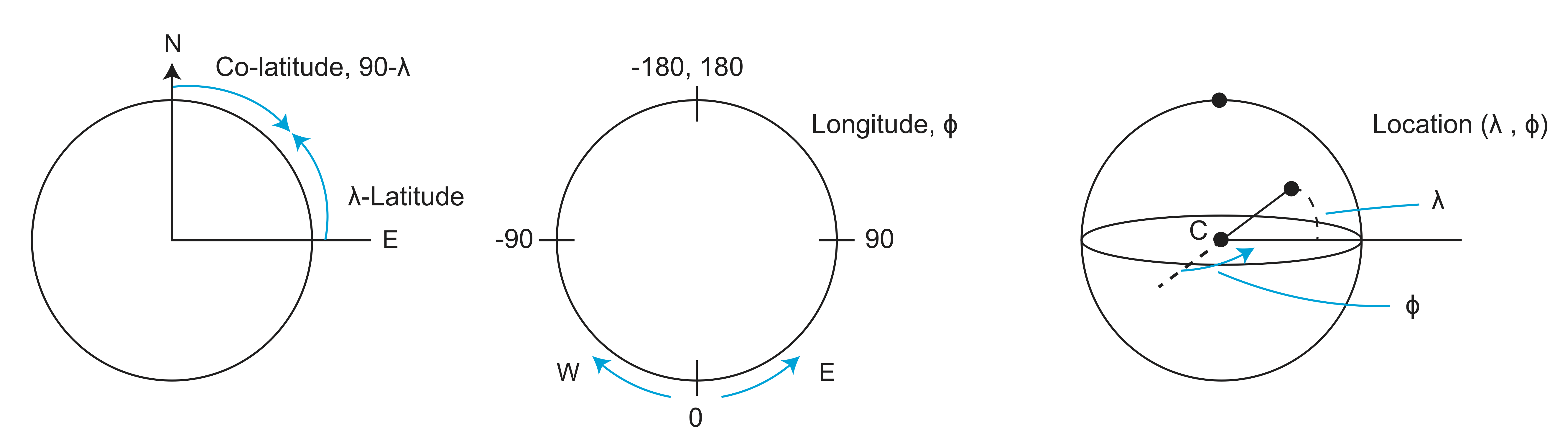
Now move point C to the top.

Figure \(\PageIndex{2}\): Point C

In all the equations below, spherical coordinates are given as \(\lambda\) (latitude) and \(\phi\) (longitude). Cartesian coordinates are given with subscripts x, y, and z, where x and y are in the equatorial plane and z points towards the north pole. The subscript p indicates a Euler Pole. A Euler Pole is typically defined by its location (\(\lambda_p,\phi_p\)) and the magnitude of the rotation, \(\omega\), in degrees/my. Latitude locations that are south of the equator should be entered as negative. Longitude locations that are west of the prime meridian should be entered as negative. Remember to convert angles to radians before using them in a cosine, sine, and tangent functions. Similarly, you need to convert the output of an inverse cosine, inverse sine, or inverse tangent from radians to degrees.

• Converting Cartesian to Spherical Coordinates

\[ \begin{align*} A_x&=\cos(\lambda)\cos(\phi) \\[4pt] A_y &=\cos(\lambda)\cos(\phi) \\[4pt] A_z &=\sin(\lambda) \end{align*}\]

• Converting Spherical to Cartesian Coordinates

\[\lambda=\sin^{-1}(A_z)\]

\[\phi=\tan^{-1}(\frac{A_y}{A_x})\]

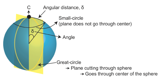
• Convert Angular Distance Between Locations

1. Convert the coordinates of each location from Spherical to Cartesian (see above). The Cartesian coordinates define a vector \(A=[A_x,A_y,A_z]\) from the center of the Earth to the location on the Earth's surface.
2. Use the dot product (or projection) of the two vectors to determine the angular distance, \(\delta\) between the two points on the surface of the Earth:

\[\delta=\cos^{-1}(A\cdot B)\]

\[\delta=\cos^{-1}(A_xB_x+A_yB_y+A_zB_z)\]

• Convert a Rotation Vector (Euler Pole) from Spherical to Cartesian

\[\omega_x=\omega \cos(\lambda_p)cos(\phi_p)\]

\[\omega_y=\omega \cos(\lambda_p)sin(\phi_p)\]

\[\omega_z=\omega \sin(\lambda_p)\]

• Convert a Rotation Vector (Euler Pole) from Cartesian to Spherical

\[\phi_p=\tan^{-1}(\frac{\omega_y}{\omega_x})\]

\[\lambda_p=\tan^{-1}(\frac{\omega_z}{\sqrt{\omega^{2}_{x}+\omega^{2}_{y}}})\]

\[\omega=\sqrt{\omega^{2}_{x}+\omega^{2}_{y}+\omega^{2}_{z}}\]

• Calculate Relative Velocity and Azimuth of Plate Motion at a Location Using the Euler Pole
  • For the relative motion of the two plates (\(\lambda_p, \phi_p\)), determine the velocity (\(\frac{mm}{yr}\)) and azimuth (degrees from north) of the relative motion at the location given by \(\lambda_x, \phi_x\). Note that this calculation is defined for any point, but only makes sense if the point is on one of the two plates. The equations use a triangle defined on the surface of the sphere, with sides a, b, and c and angles A, B, and C, where C is the angle opposite to side c. The lengths of the sides are measures in degrees.

1. Calculate the angular length of side a of the triangle.

   \[a=\cos^{-1}(\sin(\lambda_x)sin(\lambda_p)+\cos(\lambda_x)\cos(\lambda_p)\cos(\phi_p-\phi_x))\]

2. Calculate the angle C

   \[C=\sin^{-1}(\frac{\cos(\lambda_p)\sin(\phi_p-\phi_x)}{\sin(a)})\]

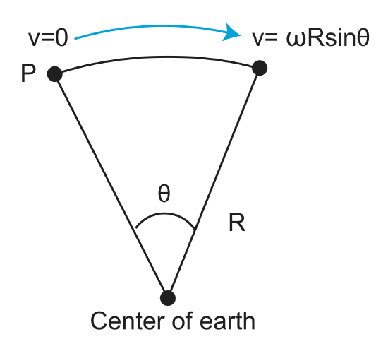
3. Calculate the magnitude of the relative velocity.

   \[v=\omega R\sin(a)\]

4. Calculate the azimuth (in degrees).

\[\beta=90+C(\frac{180}{\pi})\]

Euler Pole

Figure \(\PageIndex{3}\): Euler Pole

Figure \(\PageIndex{4}\): A-fixed vs A-moving

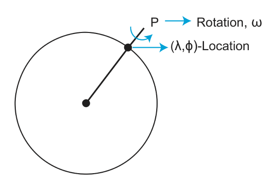
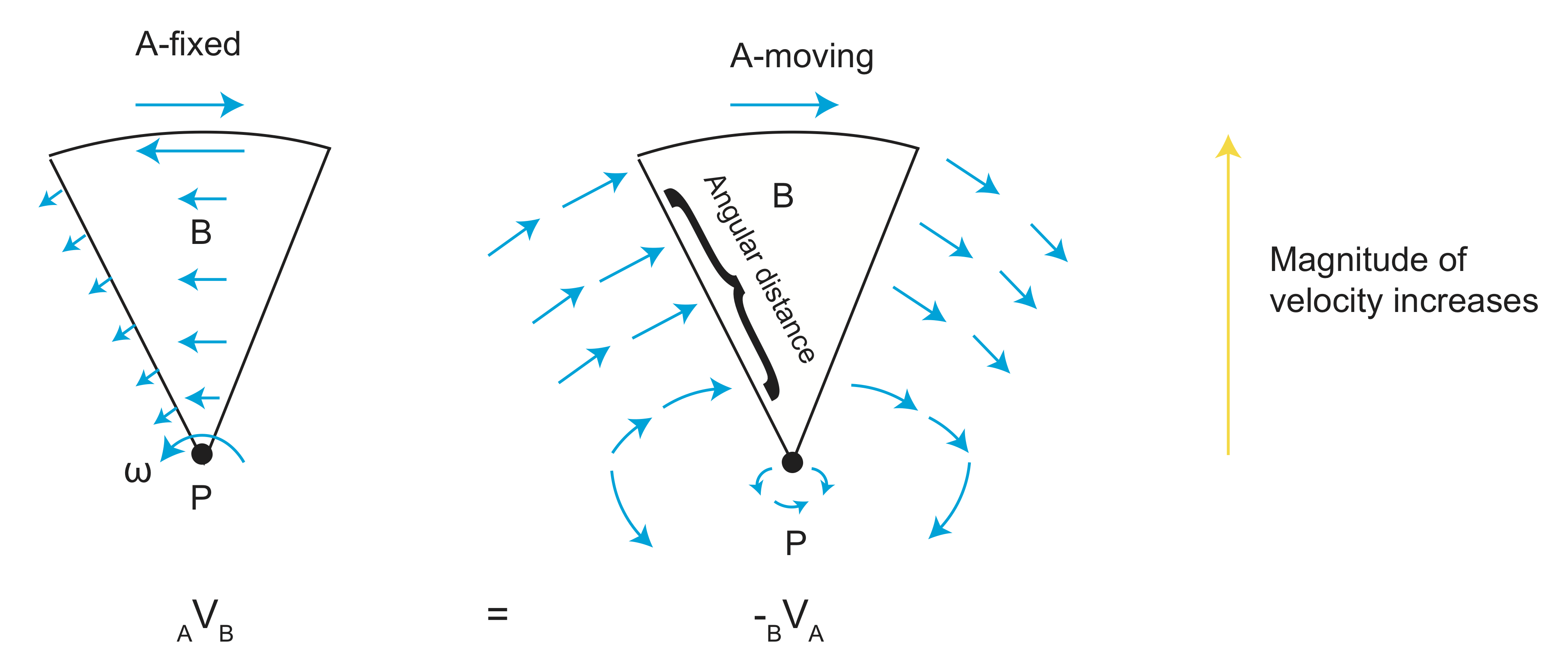
From the above figures, we can see that there is a magnitude of velocity that increases with distance from pole to 90^o.

\[v=f(\omega, distance)=\omega R sin(\theta)\]

Figure \(\PageIndex{5}\): \(v=\omega R sin(\theta)\)

Angular Distance

How do we determine angular distance? ⇒It is easier in Cartesian coordinates

Figure \(\PageIndex{6}\): Cartesian Coordinates

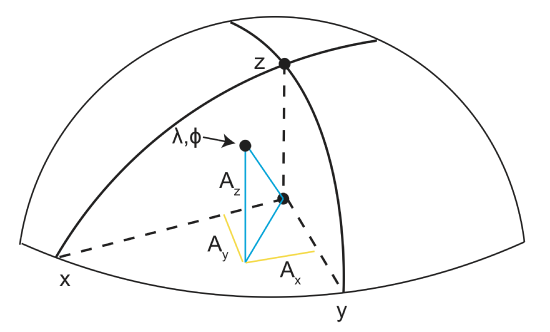
In Cartesian coordinates, the orientation on x, y, and z are very important. As we noted above, x and y are in the equatorial plane and z points towards the north pole.

If given \(\lambda_1, \phi_1\), and \(\lambda_2, \phi_2\)

1. Convert \(\lambda_1, \phi_1\)→\(A_x, A_y, A_z\)
2. Convert \(\lambda_2, \phi_2\)→\(B_x, B_y, B_z\)
3. Use dot product \(\delta=cos^{-1}(A\cdot B)\)

We can use a similar approach to express a Euler Pole in Cartesian components

\[\overset{\rightharpoonup}\omega=(\lambda_p, \phi_p, \omega)\;Spherical\;coordinates\]

This is the same as Cartesian→Spherical that we did above, but it now defines the magnitude.

\[\omega_{Cart.}=(\omega_x,\omega_y,\omega_z)\]

For plate reconstruction we need to be able to combine poles for different plates.

Example Plate Reconstruction

Given Euler Pole for \(_{PAC}\omega_{NAM}\) and \(_{PAC}\omega_{SAM}\), what is \(_{SAM}\omega_{NAM}\)? To solve this problem, what we need to do is convert the Euler Pole into something more manageable. We need components that we know how to add together. Thus, we are going to convert the Euler Pole into addable vectors, aka Cartesian components.

\[_{SAM}\overset{\rightharpoonup}\omega_{NAM}=_{SAM}\omega_{PAC}+_{PAC}\omega_{NAM}\]

Convert to Cartesian

SAM-NAM SAM-PAC PAC-NAM

\(\omega_x\) = \(\omega_x\) + \(\omega_x\)

\(\omega_y\) = \(\omega_y\) + \(\omega_y\)

\(\omega_z\) = \(\omega_z\) + \(\omega_z\)

Convert back to Spherical (see equations above)

Determine relative velocity (magnitude and direction) at a location (\(\lambda, \phi\)).

Figure \(\PageIndex{7}\): Determining Relative Velocity at Points

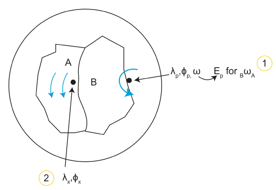
Location 1: \(\lambda_p,\phi_p,\omega\)→E_p for \(_B\omega_A\).

What is V, \(\beta\) (azimuth) at location 2? (Repeat for locations on whole plate)

Figure \(\PageIndex{8}\): Great Circles

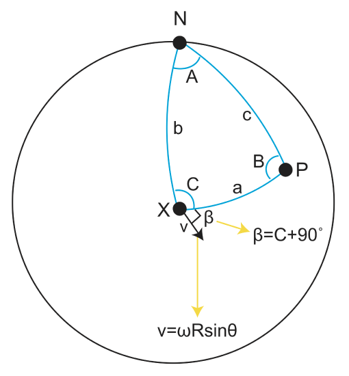
The sides a, b, c are the great circle paths, and the angles A, B, C are in the circles.

\(\beta=C+90\)

\[v=\omega Rsin\theta=\omega R sin(a)\]

\(\theta=a\), P-X angular distance

So now we need C and a. We can use known trig relations for triangles on a sphere, for example:

\[cos(a)=cos(b)cos(c)+sin(b)sin(c)cos(A)\]

\[\frac{sin(a)}{sin(A)}=\frac{sin(c)}{sin(C)}\]

Write b, c in terms of \(\lambda_p,\lambda_x\) and \(\phi_p,\phi_x\) (\(\lambda_x\) is measured from the equator)

b=90-\(\lambda_x\)

c=90-\(\lambda_p\)

A=\(\phi_p,\phi_x\) (does not depend on \(\lambda_p\))

Substitute, solve for a and c.

\[a=cos^{-1}[sin\lambda_xsin\lambda_p+cos\lambda_xcos\lambda_pcos(\phi_p-\phi_x)]\]

\[C=sin^{-1}[\frac{cos\lambda_psin(\phi_p-\phi_x)}{sin(a)}]\]

\[\beta=90+C\]

\[V=\omega Rsin(a)\]

Determining Relative Velocity at a Location

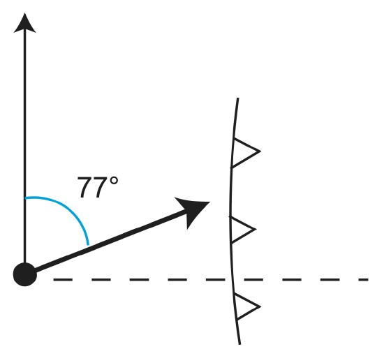
Now let's apply some real numbers determine relative velocity at a location on a plate.

Point 28^oS, 71^o W on Peru-Chile Trench

Use Nazca-South America Motion

We are given that \(\lambda_x\)=-28, \(\phi_x\)=-71, \(\lambda_p\)=56, \(\phi_p\)=94, and \(\omega\)=7.6x10^-7 degrees per year.

Plug into: a=86.26, C=-12.65^o⇒\(\beta\)=77.35^o, and finally v=8.43\(\frac{cm}{yr}\)

The plate motion can be seen in the below figure.

Figure \(\PageIndex{9}\): Motion of a Point on Peru-Chile Tench