3.2: Assignment- Using Google Earth to Visualize Plate Boundaries
- Page ID
- 12915
Module 3 Assignment
Using Google Earth to Visualize Plate Boundaries
Overview
This week you will complete an exercise on plate boundaries using Google Earth tools and any other Internet or textbook resources at your disposal. Please make sure you have completed the module reading before you complete the assignment. Please write your answers in a separate document and submit it to Assignment 1 in the Assignments Tool.
Installation
You should have the Google Earth application downloaded on your computer.
If you haven’t done that yet, please visit https://www.google.com/earth/ to download it and install it on your machine.
It is not recommended to use an iPad or a Chrome book to do this assignment.The .kmz file may not load properly and you will be unable to do the assignment.
Downloading and opening the KMZ file:
-
- Download this KMZ file: Plate Boundaries
- Launch the Google Earth application. Choose File —> Open… and navigate to the Downloads folder on your computer.
- Choose the“plate-boundaries.kmz” file to open it in Google Earth.

Instructions
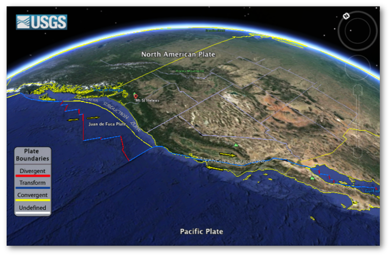
When opening the “plate-boundaries.kmz” file in Google Earth, it should automatically zoom in on the San Andreas Fault Zone in California. Take some time to acquaint yourself with the Google Earth zoom and rotation tools on the right-hand side of the window and with legend on the left side of the Google Earth window. Explore the plate boundaries in this region and across the globe. To return to the original view, simply double-click on the name of the KMZ file (“Earth’s Tectonic Plates” in the Places legend on the left-hand side of the Google Earth window). The yellow arrows indicate relative relative movement between the plates. Your current view should look like this:

West Coast Tectonics
As you have learned, the San Andreas Fault is actually a transform boundary between the Pacific and North American plates.
- Name the two plates that form the San Andreas transform fault boundary. What direction is each plate moving relative to the other?Next, zoom in on the San Andreas Fault Zone until the cities of Los Angeles and San Francisco appear on your map. (Hint: They will appear as red labeled dots. Los Angeles may appear on the map first, then zoom in a bit more and San Francisco should appear, as well).
- On which tectonic plate are the following cities located (please include one screenshot of the general area that includes at least two of these cities):
- Los Angeles, CA
- Bakersfield, CA
- San Francisco, CA
- Based on the relative motion between these two plates, is the distance between San Francisco and Los Angeles becoming greater or shorter over time? Briefly explain.Next, return to the original map view by double-clicking the name of the KMZ file “Earth’s Tectonic Plates” under the Places Legend on the left side of the Google Earth window.
- Describe the names and types of plate boundaries, as well as their relative movement, along the West coast of North America, from the Gulf of California (Sea of Cortez) northward to British Columbia, Canada.Next, zoom in on the Juan de Fuca plate, just off the coast of Washington and Oregon.
- Based on the types of plate boundaries that form the perimeter of the Juan de Fuca plate, in addition to what you have learned in the textbook about their relative rate of movement, what is the ultimate fate of the Juan de Fuca plate?
- Describe the tectonic processes that formed the Cascade Range (which includes Mt. St. Helens) in the U.S. Pacific Northwest.

Divergent Plate Boundaries
Next, zoom out and take a few minutes to explore the other plate boundaries around the globe.
- Where are most of the divergent plate boundaries located around the globe— on landmasses or in ocean basins?
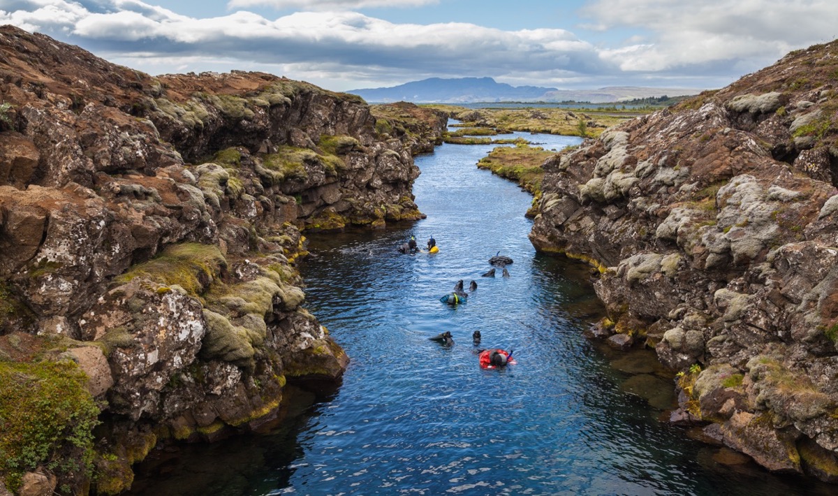
- Identify at least one location where a divergent boundary is situated in a shallow, narrow sea between landmasses. Include a screenshot.You might notice that divergent and transform boundaries often occur together in an alternating pattern. Zoom in on a region on Earth where this occurs.
- Why are mid-ocean ridges (divergent boundaries) usually offset by numerous transform faults along their length? Feel free to refer to your textbook or do some internet research (citing your sources) to determine this. Include a screenshot of the location you chose to zoom in on.
Spreading Rates
Please visit the National Oceanic and Atmospheric Administration (NOAA) website: 2008 Age of Oceans Plates)
Take a moment to study and zoom in on the map and its legend (see the screenshot of this image on the next page).
- Describe what this image is illustrating.
- Using data from the image, where is the oldest seafloor in the world and what is its age? How does this age compare to the oldest continental rocks?
- What is the reason for the discrepancy between these two ages?

- Compare the seafloor ages between the mid-Atlantic Ocean and the Pacific Ocean, off the coast of South America. Which spreading ridge is spreading faster? How does seafloor age help you determine this?
Grading Rubric
10 points: All questions were answered thoroughly and accurately. Screenshots were included where requested.
8 points: All questions were answered and were mostly accurate. Screenshots were included where requested.
5 points: Answers were too brief and a 1-2 questions were unanswered. Screenshots were not included.
2 points: Only very partial information was given. Screenshots were not included.
0 points: Did not complete the assignment.
- Assignment: Using Google Earth to Visualize Plate Boundaries. Authored by: Anne Huth. Provided by: Pima Community College. Located at: http://cc.pima.edu/~lumen/glg101/module%20parts%20-%20LUMEN/Module3/L_Assign3.html. License: CC BY: Attribution
- Figure 1: Canon Silfra, Parque Nacional de Pingvellir, Sourland, Islandia, 2014-08-16. Authored by: Diego Delso. Provided by: Wikimedia Commons. Located at: https://commons.wikimedia.org/wiki/File:Ca%C3%B1%C3%B3n_Silfra,_Parque_Nacional_de_%C3%9Eingvellir,_Su%C3%B0urland,_Islandia,_2014-08-16,_DD_055.JPG. License: CC BY-SA: Attribution-ShareAlike
- Physical Geology, Adapted by Anne Huth, Pima Community College. Authored by: Steven Earle. Located at: https://opentextbc.ca/geology/. License: CC BY: Attribution
- Laboratory Manual for Introductory Geology, Adapted by Anne Huth, Pima Community College. Authored by: Bradley Deline, Randa Harris, and Karen Defend. Located at: https://open.umn.edu/opentextbooks/BookDetail.aspx?bookId=506. License: CC BY: Attribution
- Figures 2-5: Screenshots by Anne Huth. Provided by: Google. License: All Rights Reserved


