8.3: Atmospheric Circulation

Single Cell Model

To understand the general circulation, let's create a model to simulate winds on the Earth. A model of the atmosphere is a simplified version of the Earth's Atmosphere. Let's assume Earth has no land and is entirely covered by water. Thus, wind can flow unobstructed by mountains. The Earth's rotation also adds some complexity, so for now, let's assume the Earth does not rotate and has no 23.5-degree tilt. It is still spherical, the same distance from the Sun, and the Sun's energy heats the entire globe.

On this simplified model of Earth, let's understand how large-scale winds will orient. To do that, we first need to revisit how sunlight varies with latitude. Tropical latitudes, such as the Equator, receive more direct sunlight year-round and, therefore, tend to be much warmer, while the poles receive significantly less sunlight year-round and, therefore, tend to be much colder. Since warm air rises and cold air sinks, air rises at the equator, producing low pressure along the equator all around the globe. Air also sinks at the poles, producing high pressure at the North and South poles. On Earth's surface, winds blow from high surface pressure to low surface pressure. At higher altitudes, air that rose from the surface will now return towards regions of higher surface pressure, completing a cycle of air movement.

8. Based on this model, surface winds on Earth should blow from the:
   1. Equator to the Poles
   2. Poles to the Equator

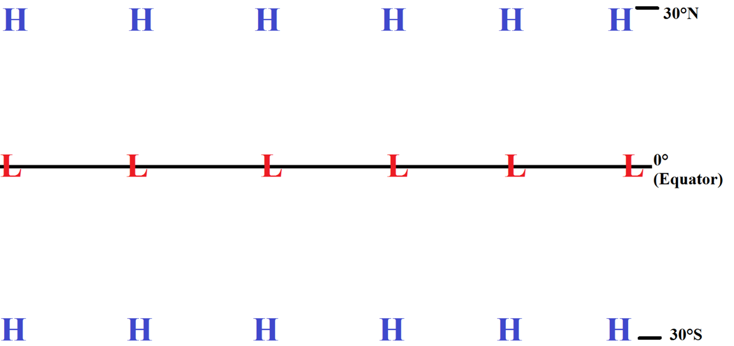
Figure \(\PageIndex{1}\) shows the Northern Hemisphere with selected latitudes indicated. You should print out or save Figure \(\PageIndex{1}\) to answer the following question.

9. Draw/label the left half of the image based on the information above and your answer to question 10. I.e., label which latitude has high pressure, which latitude has low pressure. You can draw where air is rising and where air sinks back to the surface on the left side of the figure. Please leave the right half of the image unlabeled and submit your figure.

Figure \(\PageIndex{1}\): A simplified map of the Northern Hemisphere. (CC BY 4.0; Alicia Mullens)

Congratulations, you have just constructed the single-cell model of the atmosphere! Remember, this model assumes the Earth is a uniform ball of water with no tilt or rotation. However, it’s a good first step toward modeling atmospheric circulation and accurately simulating weather at both the Equator and the Poles. However, the Earth does rotate, has a tilt, and contains land on its surface. As a result, the single-cell model can’t tell us everything we need to know. It only gives us insight into conditions at the Equator and the Poles.

Three-cell Model

Let's improve our simplified single-cell model by adding Earth's rotation. If Earth rotates, the Coriolis Force will act on any moving wind. This causes the single circulation between the equator and the poles to break up into three separate circulations.

• The Hadley Cell: Rising air over the equator travels poleward towards 30°N and 30°S, where it sinks back to the surface and returns back to the equator along the surface.
• The Ferrell Cell: Sinking air over 30°N travels northward along the surface to 60°N, where it rises up to the tropopause and then returns to 30°N at a higher altitude.
• The Polar Cell: Rising air over 60°N travels northward towards the pole (90°N), where it sinks back to the surface, and then returns to 60°N along the surface.

You should print out or save Figure \(\PageIndex{1}\), again, to answer the following question.

10. Draw/label the right half of the image based on the information above. Label which latitudes have high pressure, which latitudes have low pressure in the new three-cell model. You can draw where air is rising and where air sinks back to the surface on the right side of the figure. Remember, unlike in question 11, you'll have 3 cells this time. Finally, submit your figure.

11. The pressure systems over the Equator and the Poles are the same as in the single-cell model. However, in the three celled model, there is also a _________ surface pressure at 30°N/S and a __________ surface pressure at 60°N/S.
    1. high; low
    2. low; high
    3. high; high
    4. low; low

Congratulations, you have just drawn the three-cell model of the atmosphere! While we still haven't added land, this is a very good approximation of the surface and higher-altitude winds and pressures across the Earth. Figures \(\PageIndex{2}\) and \(\PageIndex{3}\) show the average position of high and low pressures across the planet for January and July.

Figure \(\PageIndex{2}\): Map of global mean air pressure at sea level in January. Average positions of surface high-pressure systems are shown in dark blue, while surface low-pressure systems are shown in yellow/brown. (CC BY-NC 4.0; Atmospheric pressure and wind via Encyclopedia Britannica) Alternative description of the image.

Figure \(\PageIndex{3}\): Map of global mean air pressure at sea level in July. Average positions of surface high-pressure systems are shown in dark blue, while surface low-pressure systems are shown in yellow/brown. (CC BY-NC 4.0; Atmospheric pressure and wind via Encyclopedia Britannica) Alternative description of the image.

A key consequence of this is the location of deserts and rainforests. Low pressure near the equator yields heavy rainfall, creating rainforests, while high-pressure regions at 30°N/S yield droughts, producing deserts. Figures \(\PageIndex{2}\) and \(\PageIndex{3}\) show the location of deserts and rainforests on Earth. You'll notice that it correlates well with the positions of high and low pressures on figures \(\PageIndex{2}\) and \(\PageIndex{3}\).

Figure \(\PageIndex{4}\): A map of the world's rainforests. (Public Domain; Biome Rainforest via NASA) Alternative description of the image.

Figure \(\PageIndex{5}\): A map of the world's deserts. (Public Domain; Biome Desert via NASA) Alternative description of the image.

Another interesting consequence is the formation of ocean currents, as shown in Figure \(\PageIndex{6}\). The pressure systems in Figures \(\PageIndex{2}\) and \(\PageIndex{3}\) drive global wind circulations that fuel those ocean currents.

Figure \(\PageIndex{6}\): A map of global surface ocean currents. (Public Domain; Dr Michael Pidwirny via Wikimedia Commons) Alternative description of the image.

Trade Winds

A key consequence of the general positions of high and low pressure around the world is the presence of prevailing (meaning almost permanently present) wind patterns. There are several key wind patterns in the atmosphere (such as the Jet Stream), but one of the most important is the Trade Winds. Based on the three-cell model, there is low pressure at the equator and high pressure at 30°N and 30°S. Figure \(\PageIndex{7}\) is a simplified map showing a band of high pressure at 30°, and low pressures at the Equator.

Figure \(\PageIndex{7}\): A map of surface high-pressure systems at 30° N and S, and low-pressure systems at the Equator. (CC BY 4.0; Alicia Mullens) Alternative description of the image.

12. The Pressure Gradient Force should direct the surface wind:
    1. from the equator to the 30° N and S
    2. from 30° N and S to the equator

13. In the Northern Hemisphere, the Coriolis Force, which directs winds to the right (of the direction the wind is moving, not yours), would turn the wind to the _____.
    1. East
    2. West

14. Meanwhile, in the Southern Hemisphere, the Coriolis Force, which directs winds to the right (of the direction the wind is moving, not yours), would turn the wind to the _____.
    1. East
    2. West

15. This results in a band of winds that travel ______ along the equator.
    1. east to west
    2. west to east

16. Print out or save Figure \(\PageIndex{7}\). Draw arrows to show these winds based on your answers to questions 15-18. Submit the figure.

These winds are called the Trade Winds. These constant winds in the tropics enabled early European sailors, explorers, and traders to travel across the Atlantic and Pacific oceans towards the Americas. They also transport nitrate- and phosphate-rich Saharan dust to Latin America and Brazil, where the Amazon rainforest benefits greatly from these nutrients. They promote the upwelling of cold, nutrient-rich waters off the coast of Peru and monsoons in East Asia.

However, every few years, something changes in the Equatorial Pacific. The Trade winds weaken, and the equatorial counter current strengthens. Whenever this happens, weather extremes such as droughts, floods, and heatwaves affect people across different continents. While South American countries like Chile and Peru face flooding, Australia and East Asia suffer from droughts and Heatwaves. In Africa, eastern countries like Kenya suffer from increased rainfall and deadly diseases, while southern countries, such as South Africa, face drought. Even Europe is not spared, with northern countries facing colder-than-average winters and southern countries experiencing heavier-than-average rainfall and flooding. In the next section, let's explore this global climate phenomenon that wreaks havoc across the planet.