12.5: Recent Climate Change

Changes Over the Past 100 Years

Although Earth’s climate is currently changing rapidly relative to past changes, in most regions where we live, changes are slow enough that we do not notice them directly during our daily lives. However, older people may have observed changes over their lifetimes, and in some regions, these changes are larger and more pronounced than elsewhere. In this section, we will discuss observations from the past 100 years and data from regions susceptible to climate change, where the most dramatic effects have occurred. This will not be a comprehensive documentation of existing observations. Additional observations will be discussed throughout the remainder of this book.

The Climate System

Earth’s climate system consists of interacting components, as depicted in Fig. \(\PageIndex{1}\). The atmosphere, which is the air and clouds above the surface, is about 10 km thick (more than two-thirds of its mass is contained below that height). The ocean covers more than two-thirds of Earth’s surface and has an average depth of roughly 4 km. Contrast those numbers with Earth’s radius, which is approximately 6,400 km, and you’ll find that Earth’s atmosphere and ocean are very thin layers compared to the size of the planet itself. In fact, they are about 1,000 times thinner. They are perhaps comparable to the outer layer of an onion or to the water on a wet soccer ball. Yet all life is constrained to these thin layers. The major ocean basins are the Pacific, Atlantic, Indian, and Southern Oceans. The Cryosphere comprises ice and snow, including sea ice, mountain glaciers, and ice sheets. Sea ice is frozen seawater, up to several meters thick, floating on the ocean. Ice sheets on land, composed of compacted snow, can be several kilometers thick. The Biosphere includes all living things on land and in the sea, from the smallest microbes to trees and whales. The Lithosphere, which is the solid Earth (upper crust and mantle), could also be considered an active part of Earth’s climate system because it responds to ice load and influences atmospheric carbon dioxide (CO2) concentrations and climate on long timescales through continental movements.

Figure \(\PageIndex{1}\): A composite image of Earth from space. It shows all four components of Earth’s climate system. The atmosphere has its complex cloud patterns. The ocean covers about 70% of Earth’s surface. The cryosphere is visible as the white areas on the top: sea ice covering the Arctic Ocean and the Greenland ice sheet. Green colors on land and turquoise shades along the ocean margin indicate the biosphere, including forests and phytoplankton blooms. Notice the thin layer of the atmosphere surrounding Earth in the lower left. (Public Domain; The blue marble via NASA)

The components interact by exchanging energy, water, momentum, and carbon, creating a deliciously complex coupled system. Imagine water evaporating from the tropical ocean heated by the sun. The air containing that water rises and cools, which causes the water vapor to condense into a cloud. The cloud is carried by winds over land where it rains. The rain sustains a forest. Trees are dark, having a low albedo. This influences the amount of sunlight absorbed by the Earth. Dark surfaces absorb more sunlight and warm up more than bright surfaces, such as desert sand or snow. Air warmed by the surface rises, affecting the wind.

Atmosphere

Observations indicate that the global climate is changing. Surface air temperature data, averaged over the whole Earth, indicate warming of 0.7-0.9°C over the last ~100 years, as shown in Figure \(\PageIndex{2}\). But that warming was neither steady nor smooth. From 1880 to about 1910, there was cooling, followed by warming until about 1940. After this slight cooling, approximately constant temperatures were observed until the 1970s, after which temperatures rose rapidly to the present. Each year’s temperature differs slightly from the next. Not all of these year-to-year changes are currently understood, but natural variations, which humans do not cause, do play a role. For instance, strong El Niño years, such as 1997-98 or 2015, are particularly warm, whereas La Niña years, such as 1999-2000 or 2011, are relatively cool. El Niño and La Niña are also known together as ENSO (El Niño/Southern Oscillation). ENSO is a climate variability pattern occurring in the tropical Pacific that also impacts many other regions of the Earth.

Figure \(\PageIndex{2}\): Yearly surface temperature from 1880–2025 compared to the 20th-century average (1901-2000). Blue bars indicate cooler-than-average years; red bars show warmer-than-average years. (Public Domain; Global Time Series via NOAA/NCEI)

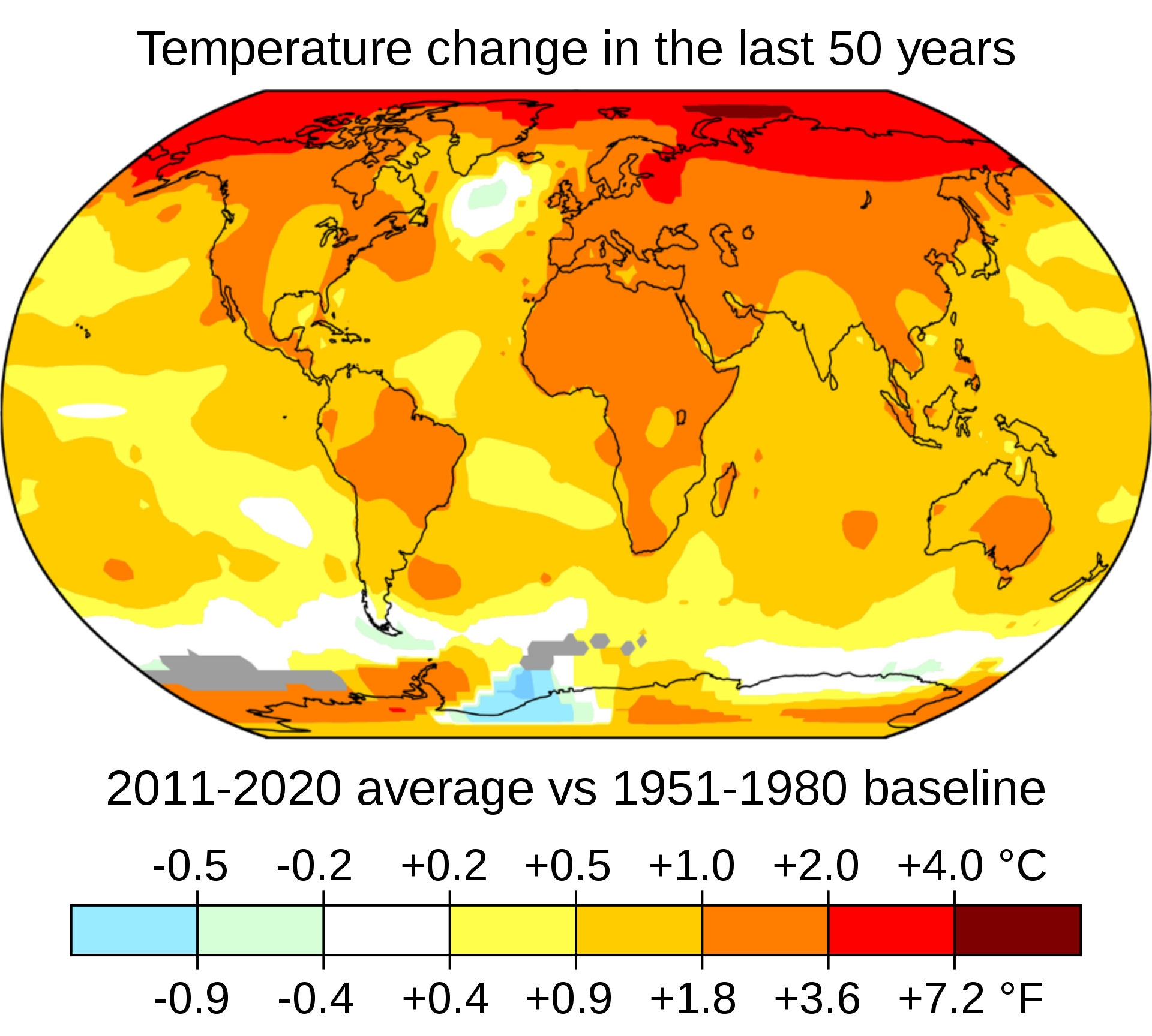
The increase in atmospheric temperatures over the last 100 years has not been uniform worldwide. Figure \(\PageIndex{3}\) shows that temperatures over land changed more than over the oceans, and the Arctic warmed more than the tropics. These patterns, called land-sea contrast and polar amplification, are pretty well understood and simulated in climate models, as we will see later. The warming is indeed almost global. The only exception is the northern North Atlantic, which has been slightly cooling for reasons we will discuss later.

Figure \(\PageIndex{3}\): Global map of recent surface temperature change shows that the warming is not uniform. Higher latitudes are warming faster than the tropics, while some oceanic regions are cooling. (CC BY-SA 4.0; NASA via Wikimedia Commons)

Analysis of thousands of temperature records into an estimate of global mean temperature change, such as Fig. \(\PageIndex{2}\), is not trivial. Issues such as changes in station locations, instrumentation, and data coverage have to be taken into account. Thus, there are a few other groups around the world that calculate global average surface temperatures, e.g. the National Aeronautics and Space Administration’s (NASA) Goddard Institute for Space Science (GISS), the Climate Research Unit (CRU) of the University of East Anglia, or the Berkeley Earth Surface Temperatures (BEST), and all come to very similar results. Errors due to unequal sampling have been estimated at approximately 0.2°C during the early part of the record and decreasing to 0.1°C during the more recent period. The fact that five groups analyzing the data with different methods reach the same conclusions suggests that the results are robust. The data's reliability has been demonstrated, and station locations (e.g., urban versus rural) don’t matter.

The global warming trend has increased the likelihood of warm and extremely warm temperatures and decreased the likelihood of cold and extremely cold temperatures. E.g., extremely warm (more than 3°C above the 1951 to 1980 average) summer temperatures over Northern Hemisphere land areas had only a 0.1% chance of occurring from 1951 to 1980. In contrast, during the decade from 2005 to 2015, the chance of those extreme warm temperatures occurring was 14.5%. Conversely, relatively cold summer temperatures (about 0.5°C cooler than the 1951-1980 average) that occurred about every third year from 1951 to 1980 occurred only 5% of the time during 2005 to 2015.

Cryosphere

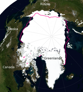
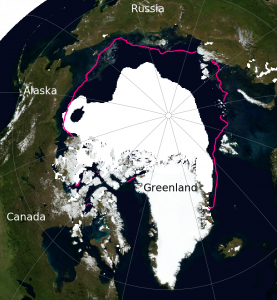
One of the most sensitive regions to climate change is the Arctic. Sea ice cover there has decreased dramatically over the past 40 years, particularly in late summer (Figure \(\PageIndex{4}\)). Arctic sea ice experiences a strong seasonal cycle. In late winter, it covers about 15.4×10⁶ km² and decreases to about 6.4×10⁶ km² in late summer, as depicted in Figure \(\PageIndex{5}\). Therefore, the relative changes are larger in late summer, with a reduction of about 46 % or 2.9×10⁶ km² from 1980 to 2015. In winter, the reduction was only about 9 % or 1.5×10⁶ km². The lost area of summer Arctic sea ice is more than 10 times the size of Oregon (255,000 km²) or four times the size of France (~650,000 km²).

A

B

Figure \(\PageIndex{4}\): Arctic sea ice extent in September 1979 (A) and 2020 (B) from satellite observations. The purple line denotes the median ice extent for 1981-2010. In 1979, the ice extent was 7.1 million square kilometers; in 2020, it was 3.9 million square kilometers. (Public Domain; Sea ice extent via NOAA/NSIDC)

In the Antarctic, sea ice undergoes a larger seasonal cycle, but it has changed less over the last 40 years than in the Arctic. Southern hemisphere sea ice has slightly increased by about 12 % or 0.5×10⁶ km² in late austral summer and 2.4 % or 2.3×10⁶ km² in austral winter. Note that year-to-year fluctuations are larger in winter than in summer and that the long-term trends in the Arctic are much larger than the short-term fluctuations. In contrast, in the Antarctic, the long-term trends are similar to the short-term fluctuations and thus less statistically significant. A trend is statistically significant if it exceeds the errors.

Figure \(\PageIndex{5}\): Changes in late summer sea ice extent in the Arctic (top) and Antarctic (bottom), and global monthly sea ice extent (center). (Public Domain; Global Snow and Ice Report via NOAA/NSIDC). Alternative description of the image.

Globally, Earth has lost approximately 2 million square kilometers of sea ice from 1980 to 2015, representing about 10% of the total. Compare that area to that of your favorite state or country.

Mountain glaciers are also sensitive to climate change. Figure \(\PageIndex{6}\) shows an example from Muir Glacier, which has retreated dramatically since 1941. This is typical of most glaciers worldwide. In fact, only a small number of glaciers show advances, whereas the vast majority melt and retreat from the valleys into higher elevations.

Figure \(\PageIndex{6}\): Muir Glacier in Glacier Bay National Park and Preserve, Alaska. The older photograph (A) is from 1941, and the recent photograph (B) shows the Muir Glacier in 2004. (Public Domain; Glaciers via NOAA/NSIDC).

The World Glacier Monitoring Service (WGMS) has compiled information on hundreds of glaciers worldwide. Figure \(\PageIndex{7}\) shows that since 1980, glaciers in all regions have been losing mass with an acceleration of loss in recent years.

Figure \(\PageIndex{7}\): Cumulative mass balance in meters water equivalent (w.e.) of mountain glaciers decreasing steadily in the past 70 years. (CC BY-NC 4.0; Global Glacier State via World Glacier Monitoring Service). Alternative description of the image.

Ice sheets are massive, continental-scale bodies of ice and snow that cover more than 50,000 square kilometers of land. They form over thousands of years when annual snowfall exceeds melting, causing layers of snow to compact into flowing ice. The two current ice sheets on Earth are in Greenland and Antarctica, which together hold over 99% of the planet's freshwater ice. Observations from the Gravity Recovery and Climate Experiment (GRACE) satellites, which measure Earth’s gravity field with very high precision and can detect mass changes, indicate that since 2002 the Greenland ice sheet has lost approximately 4,000 Gt of mass. The Antarctic ice sheet has lost about 2,500 Gigatons as illustrated in Fig. \(\PageIndex{8}\). The melting of the Greenland ice sheet currently contributes approximately 0.8 mm/yr to global sea-level rise. Antarctica’s contribution is 0.4 mm/yr, and mountain glaciers add about 0.6 mm/yr, for a total of 1.8 mm/yr sea level rise from melting of ice, according to IPCC 2019 reports.

Figure \(\PageIndex{8}\): Changes in Antarctic (red) and Greenland (blue) ice mass in billion metric tons. The dark lines are based on more than 20 studies combined for each region. Shading shows uncertainty estimates from the various data sets that contribute to the combined average. The two “NASA JPL” lines have been added to show results from one commonly cited analysis, including seasonal variations. All estimates are centered at zero in 2002 to provide a consistent point of reference. Thus, a downward slope indicates a net loss of ice and snow. For reference, 1,000 billion metric tons is equal to about 260 cubic miles of ice—enough to raise sea level by about 3 millimeters. (Public Domain; NASA JPL via EPA). Alternative description of the image.

Oceans

Subsurface ocean temperature measurements document warming over the last 60 years. The ocean’s heat content has increased by about 30×10²² Joules during that time, as illustrated in Fig. \(\PageIndex{9}\). Before 2005, subsurface temperature measurements were more limited in space and time because they were taken from ships by lowering CTD (conductivity, temperature, depth) instruments on a cable into the ocean. Since 2005, autonomous, free-drifting Argo floats have measured temperature, salinity, pressure, and velocity of the upper 2 km of the water column. Currently, there are approximately 4,000 floats in operation, providing substantially better spatial and temporal coverage than previous ship-based measurements.

Figure \(\PageIndex{9}\): Observational estimates of global ocean heat content (0-2 km). Between 1960 and 2005, ocean temperatures were measured mainly using research ships (blue line). Since 2005, autonomous ARGO floats have increased data density in both space and time, as shown by the red and black lines. Both sets of measurements indicate that global ocean heat content has increased significantly in the last 60-70 years. (Public Domain; NASA JPL via EPA). Alternative description of the image.

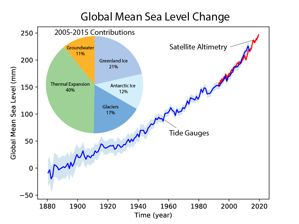
The melting of mountain glaciers and ice sheets leads to increased runoff into the ocean, which contributes to sea level rise as shown in Fig. \(\PageIndex{10}\). Sea level rise is also caused by warming sea water, which expands, and by increased runoff from groundwater pumping from aquifers. Estimates based on tide gauge records indicate that sea level has risen by approximately 20 cm from the 1870s to 2000, and by an additional 6 cm since then. The melting of mountain glaciers and ice sheets contributes approximately equally to current sea-level rise; however, if current trends continue, many mountain glaciers will likely disappear, and the large ice sheets will contribute more and more to global sea-level rise. Note that sea level rise is not spatially uniform.

Figure \(\PageIndex{10}\): Observed global mean sea level estimated from satellites (red) and tide gauges (blue). The pie chart shows the relative contributions from the melting of land ice (1.8±0.1 mm/yr), thermal expansion of seawater (1.4±0.3 mm/yr), and groundwater pumping (0.4 mm/yr; estimated as the residual) during 2005-2015 (IPCC, 2019). The total rate of sea level rise during this period (3.6±0.5 mm/yr) is larger than during earlier periods. This acceleration in sea-level rise is driven by the recent increase in melting of the Greenland and Antarctic ice sheets. (CC BY-NC 4.0; Andreas Schmittner via Introduction to Climate Science). Alternative description of the image.

Biosphere and Carbon Cycle

Plant and animal species have been observed moving poleward and upward in mountain ranges. This response is consistent with global warming and with organisms' tendency to remain within a temperature range to which they have adapted. Flowering dates of many plants have also shifted earlier in the spring, including cherry blossoms.

Figure \(\PageIndex{11}\): Atmospheric CO₂ measured at Hawaii’s Mauna Loa Observatory. The measurements were pioneered by Charles Keeling from Scripps Institution of Oceanography in 1958. (Public Domain; Global Monitoring Laboratory via NOAA). Alternative description of the image.

Carbon dioxide (CO₂) has been measured in the atmosphere since 1958 at Mauna Loa Observatory in Hawaii, as illustrated in Figure \(\PageIndex{11}\). At that time, concentrations were just below 320 parts per million (ppm). Subsequently, they increased to values of just over 424 ppm today. That is a 25% increase. Overlaid on the long-term trend is a seasonal cycle. Growth of the terrestrial biosphere in the Northern Hemisphere spring leads to CO2 drawdown and the decay of organic matter, such as fallen leaves, which increases CO₂ in the fall. CO₂ is an important greenhouse gas, and its increase over the past decades is the leading cause of the recent global warming.