12.2: Proxies

Climate Change in Earth's History

The Earth's climate is the average climate conditions of the Earth as a whole, accounting for all regional variations. For the past two centuries, our global climate has been relatively stable. People placed their farms and cities in favorable climates without considering that the climate could change. But the climate has changed throughout Earth's history, and a stable environment is not the norm.

Measurements with modern instruments (the instrumental record) are available only for roughly the past century. This is insufficient to capture the full natural variability of the climate system, making it difficult to attribute current observed changes. We seek to determine whether the recent changes are unusual relative to pre-industrial climate variability. If they are, they are more likely to be anthropogenic. If not, they could well be natural. Paleoclimate research is important for a fundamental understanding of how the climate system works. Some paleoclimate changes, e.g., ice-age cycles, were much larger than those during the instrumental record. Thus, we can learn much from paleoclimate data about the impacts of significant climate changes.

Methods

Paleoclimate research can extend the instrumental record much further back in time and has delivered a fascinating history of past climate changes. Most paleoclimate evidence is indirect and based on proxies for climate variables. This evidence is less precise than measurements from modern instruments because of additional uncertainty in the relationship between the proxy climate variable and the climate system. Examples of proxies include pollen found in lake sediments, which can be used to reconstruct past vegetation cover and, in turn, relate it to temperature and precipitation. Fossil shells of planktic foraminifera, like those depicted in Figure \(\PageIndex{1}\), can be retrieved with a coring device employed from a research vessel. Shells found deeper in the sediment are older. If shells of cold-loving foraminifera are found at a site where currently warm-loving species live, it suggests that near-surface temperatures in the past have been colder. Mathematical methods have been developed to quantify the temperature changes from the species composition. Other proxies are chemical, such as the magnesium-to-calcium ratio (Mg/Ca), which is related to temperature, or oxygen and carbon isotopes in the calcium carbonate shells of foraminifera, which can be used to reconstruct temperature, salinity, ice volume, and carbon cycling. Benthic foraminifera live on or in the ocean’s sediments and thus provide useful information on deep ocean properties.

Figure \(\PageIndex{1}\): Electron microscope pictures of Planktic and Benthic foraminifera. (CC BY-NC 4.0; Fossils via Teara)

Proxies are found in different archives such as tree rings, ice cores, corals, ocean or lake sediment cores that cover different time periods at a range of temporal resolutions, as shown in Fig. \(\PageIndex{2}\). Written historical accounts can be used to reconstruct past climatic conditions at very high temporal resolution – some ancient documents contain daily weather entries – back to about 1,000 years. Still, only a limited number of such records are available. Tree rings, corals, and speleothems (cave deposits such as stalactites and stalagmites) provide reconstructions at annual to decadal resolution back many thousands of years. Ice cores typically have decadal to centennial resolution, extending back almost a million years in Antarctica and about 100,000 years in Greenland. Ocean sediment cores span millions of years but are usually sampled at low temporal resolution, on centennial- to millennial-scale timescales.

Figure \(\PageIndex{2}\): Layered paleoclimate archives. Tree rings and corals can show annual growth rate depending on local temperature and moisture. Varves are layered sediments from lakes or seas, with light-colored layers from summer and dark-colored layers from winter. Speleotherms include cave formations such as stalactites and stalagmites, which exhibit distinct growth layers. Ice cores also provide a summer-winter color contrast similar to Speleotherms, along with trapped air bubbles detailing past atmospheric composition. (CC BY-NC-SA 4.0; Introduction to Climate Science via Oregon State). Alternative Description of Image.

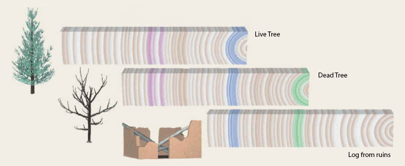
Several methods are used to date samples to construct chronologies of paleoclimate records. Tree rings are annual layers, which can be counted. Patterns of thin and thick rings can be matched from one tree to another, as illustrated in Fig. \(\PageIndex{3}\). This way, a large number of trees can be used to create a long, layer-counted chronology. Layer counting can also be used in other archives with annual layers, such as ice cores or lake sediments. Most ocean sediments don’t have annual layers because of bioturbation, which is the mixing of sediments by worms and other organisms that live in the sediment.

Figure \(\PageIndex{3}\): Climate patterns such as droughts, excessive rainfall, changes in sunlight, etc., result in certain patterns in tree trunks. Such patterns, shown in different colors, will occur at different locations in tree logs from a live tree, a recently dead tree, and an old, logged tree. Thus, long tree-ring chronologies can be constructed by matching overlapping patterns among different trees. (CC BY-NC-SA 4.0; Introduction to Climate Science via Oregon State). Alternative Description of Image.

When organic material is present, radiocarbon dating can be used to determine a sample's age. Radiocarbon (¹⁴C) decays exponentially with a half-life of 5,730 years. Thus, the lower the radiocarbon-to-carbon-12 ratio (¹⁴C/¹²C) in a sample, the older it is. This ratio can be measured precisely with a mass spectrometer. However, this method can be used only until about 40,000 years before the present, because older material contains unmeasurably small amounts of ¹⁴C.