3.4: Digital Soil Mapping

Last updated
Save as PDF

Page ID: 16621

$ \newcommand{\vecs}[1]{\overset { \scriptstyle \rightharpoonup} {\mathbf{#1}} } $ $ \newcommand{\vecd}[1]{\overset{-\!-\!\rightharpoonup}{\vphantom{a}\smash {#1}}} $$\newcommand{\id}{\mathrm{id}}$ $ \newcommand{\Span}{\mathrm{span}}$ $ \newcommand{\kernel}{\mathrm{null}\,}$ $ \newcommand{\range}{\mathrm{range}\,}$ $ \newcommand{\RealPart}{\mathrm{Re}}$ $ \newcommand{\ImaginaryPart}{\mathrm{Im}}$ $ \newcommand{\Argument}{\mathrm{Arg}}$ $ \newcommand{\norm}[1]{\| #1 \|}$ $ \newcommand{\inner}[2]{\langle #1, #2 \rangle}$ $ \newcommand{\Span}{\mathrm{span}}$ $\newcommand{\id}{\mathrm{id}}$ $ \newcommand{\Span}{\mathrm{span}}$ $ \newcommand{\kernel}{\mathrm{null}\,}$ $ \newcommand{\range}{\mathrm{range}\,}$ $ \newcommand{\RealPart}{\mathrm{Re}}$ $ \newcommand{\ImaginaryPart}{\mathrm{Im}}$ $ \newcommand{\Argument}{\mathrm{Arg}}$ $ \newcommand{\norm}[1]{\| #1 \|}$ $ \newcommand{\inner}[2]{\langle #1, #2 \rangle}$ $ \newcommand{\Span}{\mathrm{span}}$$\newcommand{\AA}{\unicode[.8,0]{x212B}}$

Brandon Heung, Daniel Saurette, and Chuck Bulmer

Learning Objectives

Upon completion of this chapter, students will be able to:

Describe and rationalize a transition from conventional soil information to digital soil information
Link theories of pedogenesis to applications of digital soil mapping
Provide an overview of how digital soil information is used to generate soil maps

INTRODUCTION

Globally, Canada has the third and seventh largest asset bases in terms of forested and arable lands; hence, accurate and precise soil information is needed to maintain and improve our soil resources and to address significant environmental challenges, such as agricultural land loss or the decline in soil organic carbon and deterioration of soil health. Without information on the spatial patterns of soil, our ability to identify the most suitable locations to realize new agricultural and resource management opportunities, and to capitalize on our natural resources will be challenged in the future.

The demand for up-to-date soil information has been increasing to address emerging environmental issues such as sustainable food production; climate change regulation, adaptation, and mitigation; soil degradation; land resource management; and the provision of earth system services across all geographical extents (Sanchez et al., 2009; FAO and Global Soil Partnership, 2016). Additionally, better soil information is necessary for performing soil assessments; and the reduction and informing of risks for decision-making (Carré et al., 2007; Finke, 2012; Arrouays et al., 2014).

Canada has a long history of soil surveying—with the first soil survey being completed in Ontario in 1914 (McKeague and Stobbe, 1978)—and maps produced from the legacy soil surveys have been used to inform land management and planning for many years. Digitized versions of legacy maps are widely available online and are still being used to this day (e.g., British Columbia’s Soil Information Finder Tool). Despite this, it has been well recognized by the soil science community that the approaches and techniques used in legacy soil survey may not be suitable for providing the precise and high-resolution information demanded by modern agricultural management and environmental assessment activities. With continued advances in computing, remote and proximal sensing technologies, and geographical information systems (GIS), soil surveying activities have transformed towards digitally-based techniques that can provide soil information that is more accurate and precise than what was previously available, and in an efficient manner.

This chapter will summarize the transition of conventional soil surveying approaches to digital soil mapping (DSM) approaches; present a theoretical framework of DSM; and provide an overview of how emerging technologies may be used to generate digital soil maps.

CONVENTIONAL SOIL MAPPING

Two major achievements contributed to the development of conventional soil survey methods in North America. The first achievement was the formalization of Hans Jenny’s Factors of Soil Formation (1941) and the second was the formalization of national soil taxonomic systems in the US (Soil Taxonomy; Soil Survey Staff, 1975) and Canada (The Canadian System of Soil Classification, CSSC; Canada Soil Survey Committee, 1978; See Chapter 8). The classification systems described how soils were classified based on morphological properties that could easily be measured and quantified in the field. Jenny’s clorpt model (Eqn. 1) characterizes the environmental conditions for which soils are found as a function of climate (cl), organisms (o), relief (r), parent material (p), time (t), and other local factors that influence soils (…):

(1) $\begin{equation*}S = f\,(cl,\;o,\;r,\;p,\;t,\;...)\end{equation*}$

The clorpt model was originally proposed as a method for studying how soils varied, quantitatively, as a function of various state factors. One of the key quotes that gets overlooked in Jenny’s book is that he describes:

“The factors are not formers, or creators, or forces; they are variables that define the state of a soil system.”

In other words, these factors are simply describing the environmental conditions from which a soil (and their properties) are found and therefore, these variables may be used as the basis for predicting soils using a model that relates the soil to the environment (i.e., soil-environmental model).

The adoption of Jenny’s clorpt model led to dramatic improvements in soil survey compared to the early efforts. Soil descriptions and maps began to be organized around the factors of soil formation, especially by organizing soils into groups based on properties of their parent material, but also by linking fine-scale topographic variation to the boundaries between soils. This provided a rationale and system for linking soil unit boundaries to topographic features.

Soil classification systems have also led to the improvement of soil surveys because they focused on the most important soil properties for field surveyors to evaluate, and these were applied consistently across multiple survey projects, allowing for better correlation over large areas.

The conceptual improvements associated with the clorpt model of soil formation and the use of standardized soil profile information, coming from the application of a uniform soil classification system, were largely responsible for what we see today as the high information value of soil survey throughout the latter half of the 20^th century. The digitization of these surveys has provided valuable information to land managers, and in some instances, it has also provided the raw material for the development of today’s digital soil maps. This would not have been possible without these advancements.

Conventional Representations of Soil

Soils may be represented in several ways: a profile, pedon, polypedon, or map unit (Figure 17.1). The soil profile is a 2-dimensional representation and the pedon is a 3-dimensional representation that typically is 1–3 m laterally and 1–2 m vertically. In principal, the properties of the pedon should not vary horizontally (only vertically) and when several similar pedons are connected, it is referred to as a polypedon. The polypedon concept differs from a map unit because the map unit, a distinct polygon that is mapped by soil surveyors, is an areal representation of a polypedon or a polypedon complex. There are two types of mapping units: consociations and associations. Consociations are map units delineated based on a single taxonomic unit or series and may be referred to as a simple mapping unit whereas associations consist of two or more dissimilar soil taxa (multiple components) that occur in a pattern that is too complex to be resolved at the selected mapping scale (Hole and Campbell, 1985; Schaetzl and Anderson, 2005). In the case of complex map units, the proportion of each soil class within the map unit is specified in the map legend or the map symbol.

Figure 17.1. Illustration of the concept of the soil pedon and soil polypedon. © Dan Pennock, Univ. of Saskatchewan is licensed under a CC BY (Attribution) license.

Producing Conventional Soil Maps

MacMillan et al. (1992) describes the steps involved in making a conventional soil map, beginning with the preliminary steps of defining the objectives, compiling background information, and initial legend development. The preliminary (primarily office based) steps are followed by soil inspections, field mapping, and correlation. Finally, the map is produced, and a report written. The procedures used to produce soil maps were documented extensively during the period when these maps were being produced in many countries throughout the world. In Canada, the procedures and considerations for meeting soil mapping objectives were documented in Mapping Systems Working Group (1981) and Coen (1987).

In a conventional survey, one key aspect of planning is to establish the survey intensity level, which expresses the amount of (field) work done, and the level of detail for the information collected. Guidelines for describing the survey intensity level are provided in Table 17.1 (Mapping Systems Working Group 1981; Coen, 1987).

Table 17.1. Soil survey intensity level guidelines adapted from Mapping Systems Working Group (1981)

Survey Intensity Level (SIL)	Common Name	Field Intensity	Method of Field Checking	Typical Publication Scale	Taxonomic Level
1	Very detailed	1 inspection per polygon	Foot traverse <0.5 km apart	1:5,000	Series
2	Detailed	1 inspection in >90% of polygons	Foot/vehicle traverse 2 km apart	1:20,000	Series or family
3	Reconnaissance	1 inspection in 60-80% of polygons	Foot/vehicle traverse 4 km apart	1:50,000	Series, family or subgroup
4	Broad Reconnaissance	1 inspection in 30-60% of polygons	Vehicle traverse 8 km apart/helicopter	1:100,000	Family or subgroup
5	Exploratory	1 inspection in <30% of polygons	Vehicle traverse 10 km apart/helicopter	1:250,000	Subgroup, great group or order

In Table 17.1, a conceptual diagram of the soil survey process is presented, where environmental data and field inspections are incorporated into soil landscape models and used to prepare a conventional soil map. The soil landscape model is a key feature of the conventional soil survey: these were mental models, which allowed surveyors to extend the information from the field inspections in one area to other areas with similar environmental characteristics, greatly improving map production at a time when access networks were more limited than they are today.

Aerial photographs, when they became widely available, were an important part of the process. In a conventional soil survey, the mapper first reviewed existing information and knowledge of soil-environmental relationships for the area. Aerial photographs were then reviewed in order to identify topographic and vegetation patterns, where the soil-environmental variables exhibited an external expression on the landscape in order to attempt the correlation of landscape characteristics to soil boundaries (soil-landscape relationships). Aerial photos became widely used during and after the 1960s, and air photo interpretation was carried out using a stereoscope, which allows the mapper to see the landscape in 3D—significantly increasing the quality of the soil maps being produced. Again, by referring to Jenny’s clorpt model (1941) the underlying hypothesis was that areas with similar soil-environmental characteristics should have similar soils. A preliminary reconnaissance map was developed by drawing boundaries between soil units, and the preliminary map was then tested in the field where morphological classification was performed on the preliminary map units and linked to a soil taxonomic unit (e.g., series). When the series were identified, the mapper attempted to further delineate or adjust the boundaries of the map unit based on where the rate of change in soil properties was the greatest and to enclose relatively uniform areas within the map units.

Supplemented with field data and profile descriptions, map units with similar morphological characteristics are grouped into the same taxonomic unit (e.g., series) and the soil properties and the range of environmental conditions, from which the soils were found, were then described in the soil legend. Conventional soil surveys were produced at varying survey intensities, which reflects the amount of detail that is shown on a map and at its corresponding map scale (Table 17.1, Figure 17.2). Large parts of Canada were mapped this way, providing essential information for the development of agriculture and natural resources.

Figure 17.2. Conceptual framework for developing conventional soil maps using local information and expert knowledge by a soil surveyor to derive soil landscape models, with the use of aerial photographs to assign soils to landscape positions. © Chuck Bulmer, BC Ministry of Forests, Lands and Natural Resource Operations is licensed under a CC BY (Attribution) license.

The Evolution of Conventional Soil Maps

Because most of the conventional soil maps that were produced in Canada up to the 1990’s were prepared for land inventory and regional planning purposes as ‘semi detailed’ maps, and because they were produced using analogue cartographic techniques (i.e., producing a hard copy map), they have certain limitations when compared to the current need for high resolution products. The chloropleth map representation used to present soil information on paper maps, and the lack of technology available at the time to acquire and process digital gridded soil and terrain data, are two key aspects of these limitations.

Firstly, the data in a chloropleth map is represented as discrete classes where the conditions are assumed to be homogenous within the map unit (Hole, 1978). Furthermore, it is also recognized that a significant amount of spatial generalization (i.e., simplification) within the map unit occurs due to inclusions of subdominant soils that are too small to be mapped at the map scale (Hole and Campbell, 1985). As a result, the purity of the mapping units is closely related to the complexity of the terrain, external expression of boundaries, survey effort, and mapping scale (Beckett, 1971). Although it would be ideal to have a soil map that consists of only simple mapping units, increasing the proportion of ‘pure’ map units within a map has been shown to result in an exponential increase in cost for developing the map (Bie et al., 1973).

Other issues may be related to the imprecision in map unit boundaries where the variability (or lack thereof) of the soil’s surface does not necessarily coincide with the variability that may be occurring belowground (Hole, 1978). In addition, the changes in soil are not necessarily discrete (as suggested by the use of boundaries), but rather, they are fuzzy where the soil attributes between two neighbouring map units are an intergrade of the soil properties of the two units (Zhu and Band, 1994; Schaetzl and Anderson, 2005).

The final set of challenges stem from the delineation of map units based on the mental-models of soil-environmental relationships that were developed primarily to coincide with the objectives for a specific map product and area. These objectives varied from one map to another, and although they normally were described in the survey report, they are rarely suitable for incorporation into computer-based soil assessments spanning large areas with several smaller surveys. Consequently, inconsistencies manifested themselves in soil maps as mismatched boundaries of map units amongst different counties, states/provinces, and countries (Figure 17.3; Thompson et al., 2012; Dewitte et al., 2013). In addition, inconsistencies may also lead to problems such as having multiple soil series with the same soil properties, which results in redundancy, or even worse, where two soil series with the same name have completely different soil properties (Thompson et al., 2012).

Despite these limitations, in many parts of Canada and the world, legacy soil maps incorporate vast amounts of information derived from field inspections and soil surveyor knowledge. For these reasons, they represent an important source of training data for the development of digital soil maps to meet current needs.

Figure 17.3. Mismatched soil survey boundaries at the intersection of Durham, Northumberland, and Peterborough counties in Ontario. © Daniel D. Saurette, Ontario Ministry of Agriculture, Food and Rural Affairs is licensed under a CC BY (Attribution) license.

DIGITAL SOIL MAPPING

Soil surveying, as a practice, has been evolving to take advantage of the advancements in computing technology (Minasny and McBratney, 2016; Rossiter, 2018), remote-sensing technologies (Mulder et al., 2011), proximal-sensing technologies (Viscarra Rossel et al., 2011), GIS, machine-learning techniques (Heung et al., 2016), and the increasing availability of geospatial datasets (McBratney et al., 2003; Minasny and McBratney, 2016; Scull et al., 2003). Hence, pedometrics—a branch of soil science that applies “mathematical and statistical methods for the study of the distribution and genesis of soils” (Webster, 1994)—has been an emerging field of research, globally. Although pedometric techniques for producing digital soil maps (DSM) have existed since as early as the 1970s (e.g., Webster and Burrough, 1972a, 1972b), technological advances have facilitated the production of DSM products since the 2000s (McBratney et al., 2003; Scull et al., 2003; Minasny and McBratney, 2016). Furthermore, these advances have also allowed for soil maps to be produced for progressively larger areas and in increasing levels of detail (Minasny and McBratney, 2016).

Some of the major achievements that have been made by pedometricians around the world have included, but are not limited to, the establishment of GlobalSoilMap.net, an international organization that aims to coordinate and produce global-scale digital soil maps; and the establishment of SoilGrids.org, an organization that was the first to develop a suite of global-scale map products. Within Canada, this is still an emerging and evolving area of research within the agricultural, forestry, and environmental sectors since 2010. With great success, the DSM community has been providing valuable information at multiple spatial scales to various stakeholders, including landowners, farmers, governments, and forest managers.

The steps for digital soil map production (after Kienast-Brown et al. 2017) are compared with those for conventional maps in Figure 17.4. The two methods of map development share several common steps, especially the need for detailed field inspections and an ability to correctly describe and interpret soil profile data. For digital soil maps, specifications for information content and level of detail are defined by the target spatial resolution, where the level of detail is inferred, and in the training data step, where the modeled attributes are defined. Some organizations have developed mapping specifications for digital soil map production (e.g., FAO and Intergovernmental Technical Panel on Soils, 2018).

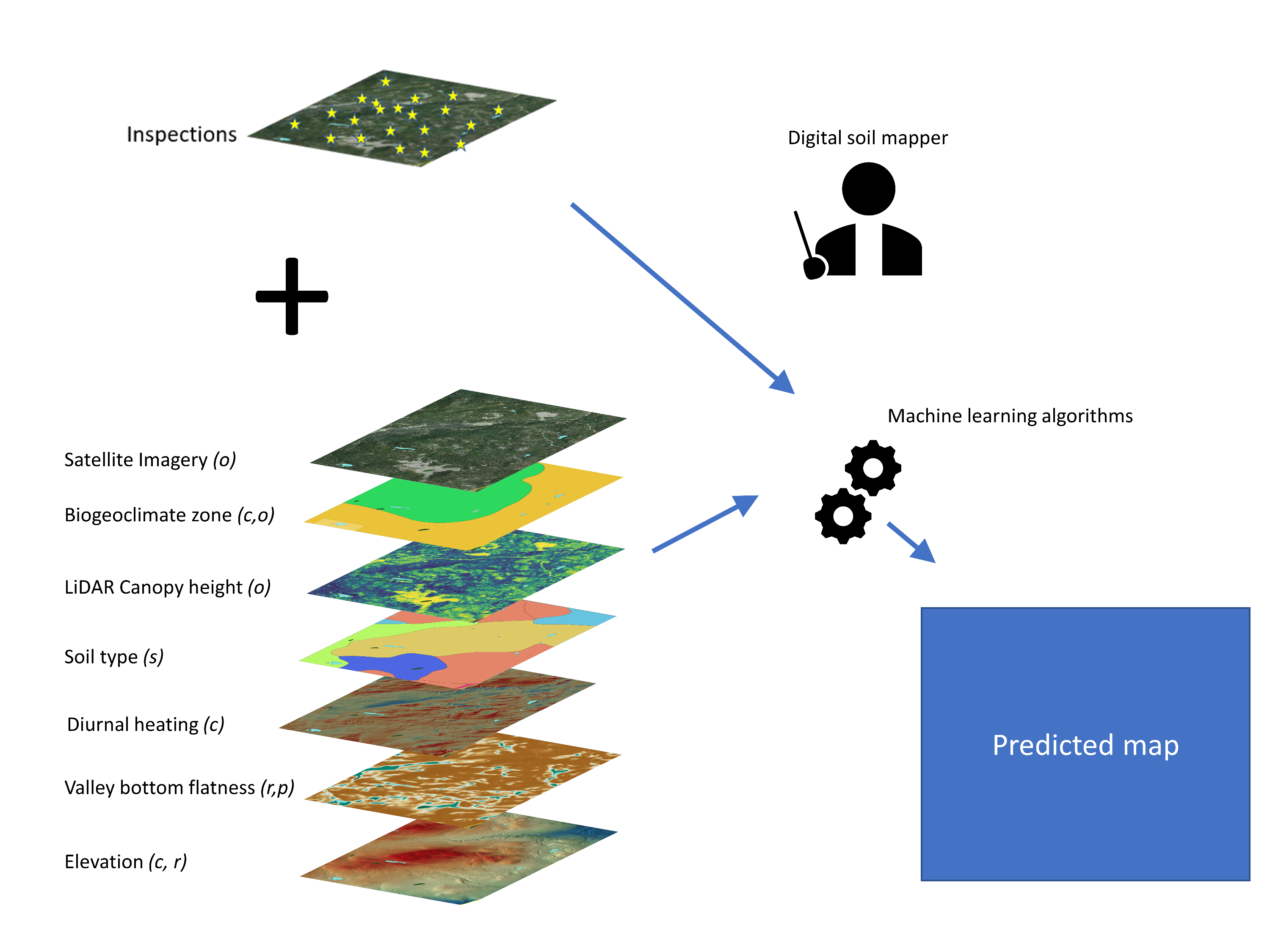
Conventional and digital soil mapping differ primarily in the way that soil classes or attribute values are assigned to locations. In conventional soil mapping, a combination of field inspection, extrapolation and expert knowledge is used, while in digital soil mapping, field information and quantitative inference models are used to predict soil conditions at given locations. The conceptual framework for DSM, presented in Figure 17.5, highlights the role that machine learning algorithms play in the production of a digital soil map. Of critical importance is the need for field inspection data in both conventional and digital soil mapping approaches—DSM does not remove the need for trained pedologists and soil surveyors—the primary difference is in how the field data is used to construct the soil maps.

Figure 17.4. Steps in production of conventional and digital soil maps. Adapted from MacMillan et al. (1992) and Kienast-Brown et al. (2017). © Adapted from MacMillan et al. (1992) and Kienast-Brown et al. (2017). adapted by Chuck Bulmer, BC Ministry of Forests, Lands and Natural Resource Operations is licensed under a CC BY (Attribution) license.

Figure 17.5. Conceptual process of creating a digital soil map, where the development and use of the soil landscape model are no longer held exclusively as mental models of the soil surveyor, and the digital soil mapper must assume the role of a conductor, guiding the process of supplying field inspection and environmental data (i.e., the training data) to algorithms that then assign soil classes and attributes to landscape positions. © Chuck Bulmer, BC Ministry of Forests, Lands and Natural Resource Operations is licensed under a CC BY (Attribution) license.

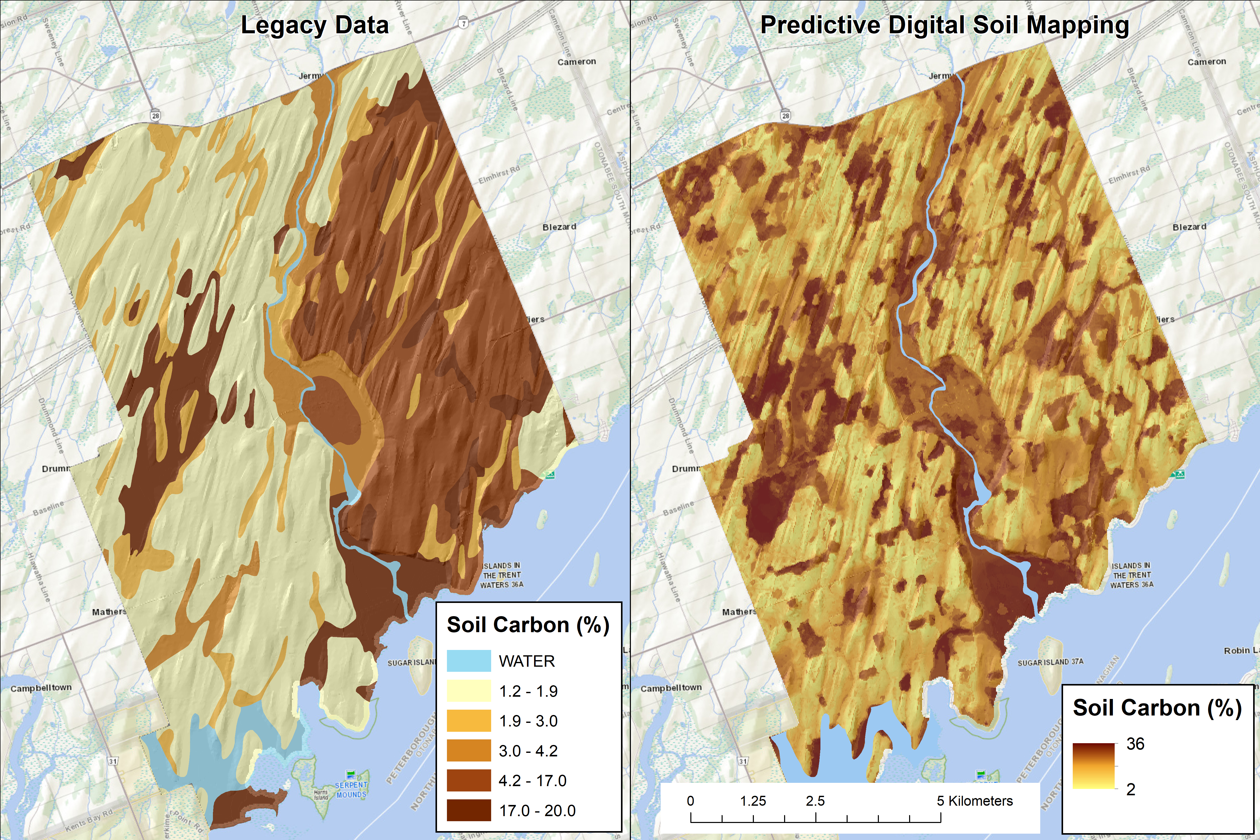
It is important to recognize that whereas conventional soil maps represent soil map units using polygons, DSM aims to produce maps using a raster representation. Raster data consist of a grid of two-dimensional cells (i.e. pixels), whereby each cell has a geographical location (e.g., longitude and latitude) and a corresponding value of a variable. Figure 17.6 shows a comparison of a conventional soil map that is represented in the polygon format, and a digital soil map that is represented in the raster format. Within DSM, the raster data may represent soil attributes (e.g., soil pH), a soil class (e.g., drainage class), or one of the environmental factors that are used to make spatial predictions of soils.

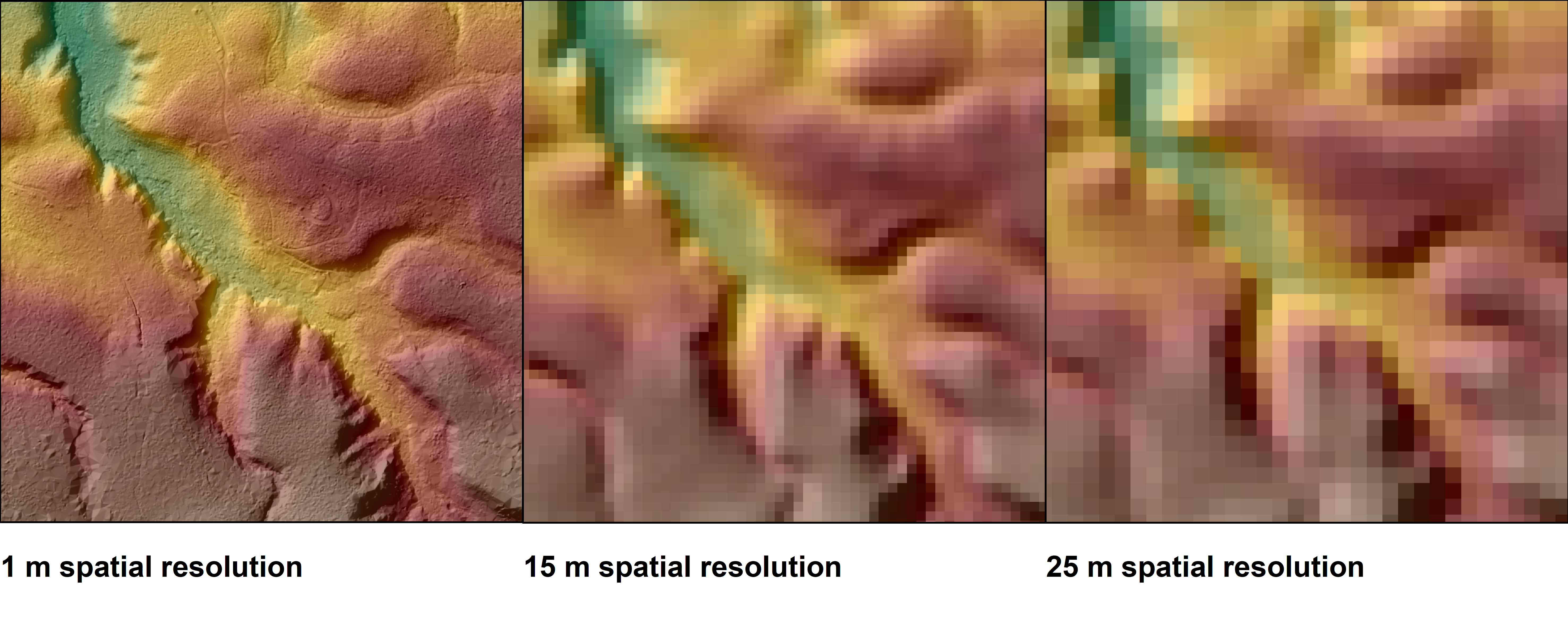
Figure 17.6. Comparison of a soil organic carbon (%) map digitized from a conventional soil survey map (left) and predictive digital soil map at a 20 m spatial resolution for the Keene area, Peterborough County, Ontario. © Daniel D. Saurette, Ontario Ministry of Agriculture, Food and Rural Affairs is licensed under a CC BY (Attribution) license.

Critical to the raster data representation is the concept of spatial resolution; i.e., the dimension of each cell with respect to the area that it is representing on the ground. For example, a spatial resolution of 10 m will indicate that each grid cell or pixel will represent a 10 × 10 m area on the ground. Ultimately, the spatial resolution will determine the level of detail or precision of a soil map and its uses. For example, a fine- or high-resolution map (e.g., 5–10 m spatial resolution) may be more useful for representing soil variability of individual agricultural fields for precision agricultural purposes whereas a coarse- or low-resolution map (e.g., 250–1,000 m spatial resolution) may be more practical for representing global-scale soil variability and the integration of that data into global climate models. Therefore, when selecting an appropriate spatial resolution, a soil mapper needs to consider what that map is used for and the spatial resolution of the input data that is required to generate those maps.

Of course, there is also a trade-off between spatial resolution and data size whereby higher resolution data are larger in size than lower resolution data. For example, when the spatial resolution is increased by a factor of two (e.g., decreasing the cell size from 10 × 10 m to 5 × 5 m), the size of the dataset could be increased by a factor of four because four pixels are now required to represent the same area as the original pixel. Figure 17.7 shows the relationship between spatial resolution and detail for topographic data.

Figure 17.7. Digital elevation model produced at 1 m, 15 m, and 25 m spatial resolutions. Original data was acquired from the Nova Scotia provincial LiDAR dataset. © Brandon Heung, Dalhousie University is licensed under a CC BY (Attribution) license.

The scorpan Model

Despite the wide use of Jenny’s (1941) clorpt model, it is still largely a conceptual model; however, if we refer to his quote, we should recall that the clorpt factors are variables that describe the environment. To apply digital approaches, we need to recognize that these clorpt factors may also be represented using GIS—a computerized system that is able to acquire, store, analyse, and visualize spatial data. To fully make the theoretical transition from conventional to digital soil mapping approaches, McBratney et al. (2003) proposed the scorpan model as an extension of the clorpt model in the following:

(2) $\begin{equation*}S = f\,(s,\;c,\;o,\;r,\;p,\;a,\;n)\end{equation*}$

The scorpan model shares the same variables as the clorpt model, which includes climate (c), organisms (o), relief (r), parent material (p), and time/age (a). The additional variables include s, which represents the intrinsic properties of the soil (e.g., the spectral properties of the soil) that may be captured by various remote and proximal sensors; and n, which represents the spatial coordinates of a sample or the location relative to another geographical phenomenon (e.g., distance to river). Here, individual scorpan factors, or a combination of them, are used to predict the distribution of a soil property or soil class, S, of interest using a quantitative function, f (), that represents the soil-environmental relationship.

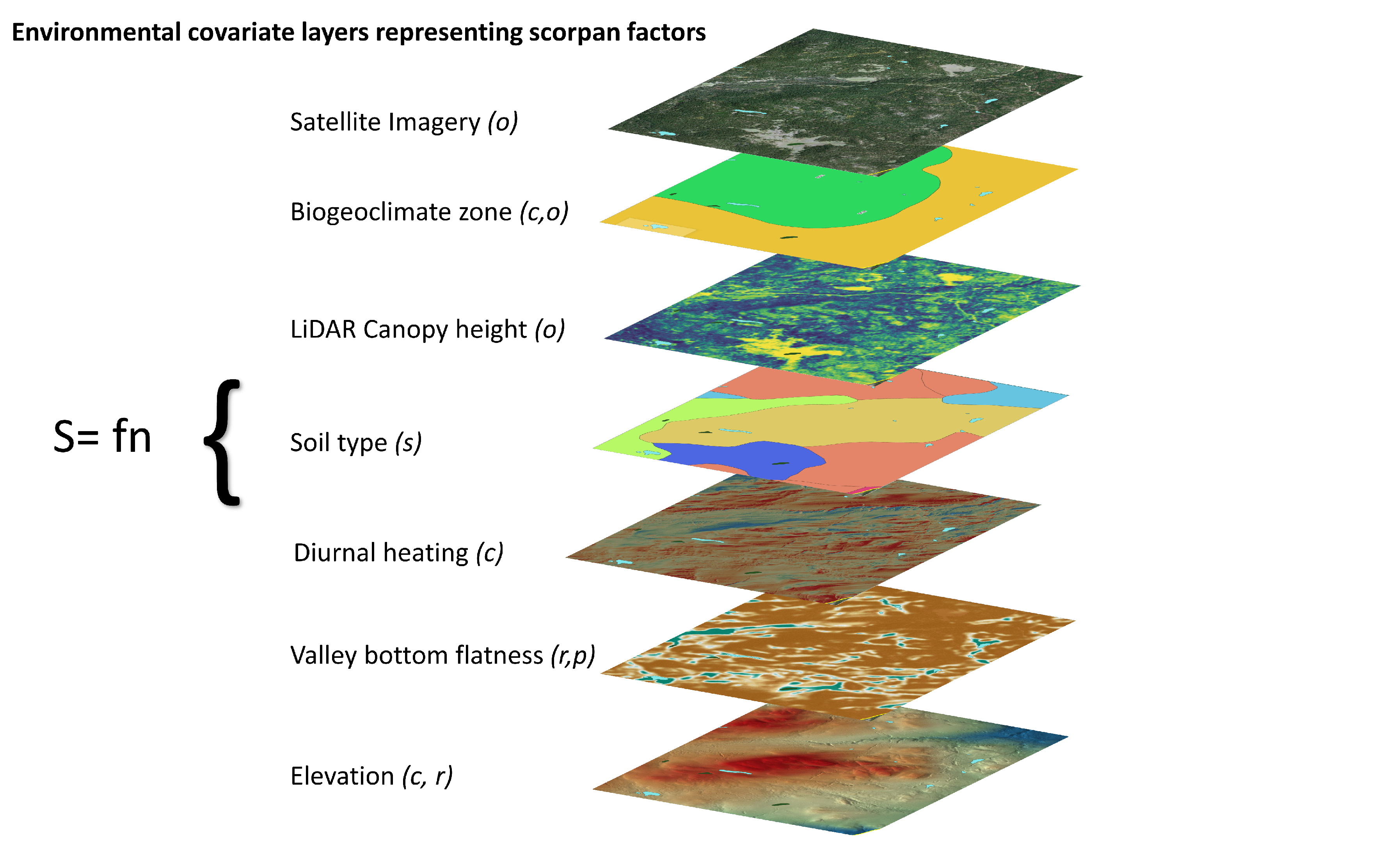
Representing the scorpan Factors

The effectiveness of the scorpan model is in its flexibility to integrate data from existing soil surveys and geospatial datasets acquired from multiple sources, such as remote sensing data, digital elevation data, climate data, land use data, and geological data (McKenzie and Ryan, 1999). These scorpan factors are represented in the raster format and therefore, each dataset also has a corresponding spatial resolution and projection system. Hence, each individual dataset may need to be re-projected into a common projection system and scaled to a uniform spatial resolution so that all the individual cells of the various datasets are spatially aligned (Figure 17.8).

The following provides a brief overview of the scorpan factors.

Figure 17.8. Representation of scorpan factors within a raster format. © Chuck Bulmer, BC Ministry of Forests, Lands and Natural Resource Operations is licensed under a CC BY (Attribution) license.

Soil (s)

The s factor is the second most frequently used factor in DSM studies (McBratney et al., 2003). Again, the s factor is founded on the concept that soils may be used to predict soils and therefore there are multiple sources from which this data may be acquired from: conventional soil survey data, proximal soil sensors, and remote sensors.

Conventional Soil Survey: Conventional soil maps represent a wealth of information derived from many years of field work by previous generations of soil scientists, and therefore they are extremely valuable sources of information that can be used for prediction purposes due to the relationship that different soil variables have with each other. For example, Paul et al. (2020a; 2020b) used the Soils of the Langley-Vancouver Map Area (Luttmerding, 1980) to generate digital layers of sand, silt, and clay percentages; and cation exchange capacity that were then used as predictors for mapping soil organic carbon and soil workability for the Lower Fraser Valley, BC. In both studies, predictors generated from the original conventional soil survey were identified as the most important layers. Although soil surveying approaches have transitioned to digital techniques, conventional soil maps should not be disregarded because they remain a valuable and complementary source of information within a DSM framework.

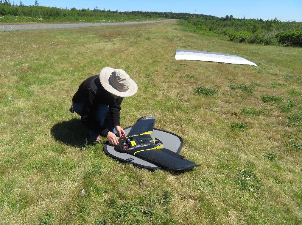
Remote Sensors: Remote sensors are designed to take measurements of the Earth’s surface without any physical contact and are therefore mounted on an aircraft or a satellite. Here, it is important to recognize that data acquired from remote sensing could be used to represent multiple scorpan factors. Within the suite of remote sensors, spectral sensors (e.g., multispectral, hyperspectral) that detect reflected or emitted energy from the electromagnetic spectrum are most used in DSM (McBratney et al., 2003; Mulder et al., 2011). For example, Landsat 8 provides measurements for visible (e.g., red, green, blue wavelengths) and infrared (e.g., near infrared, short wavelength, and long wavelength) light. Alternatively, various spectral sensors may also be mounted on an aircraft or a remotely piloted aerial system (RPAS) if higher spatial resolution data is required (Figure 17.9).

There are several issues related to the use of spectral sensors for DSM purposes, especially given that soil measurements are often obscured by vegetation. Furthermore, atmospheric effects and topographic distortions may cause anomalous measurements. In addition, when using spectral sensors, one needs to consider the day and time of which the imagery is taken. Lastly, remote sensors generally only acquire data that are representative of surface soils (5–6 cm; Adamchuk et al., 2017). Despite these issues however, under bare-soil conditions, measurements of the spectral properties of the soil have shown to correspond well with soil properties such as soil mineralogy, texture, soil organic matter, soil moisture, and other soil properties (Mulder et al., 2011).

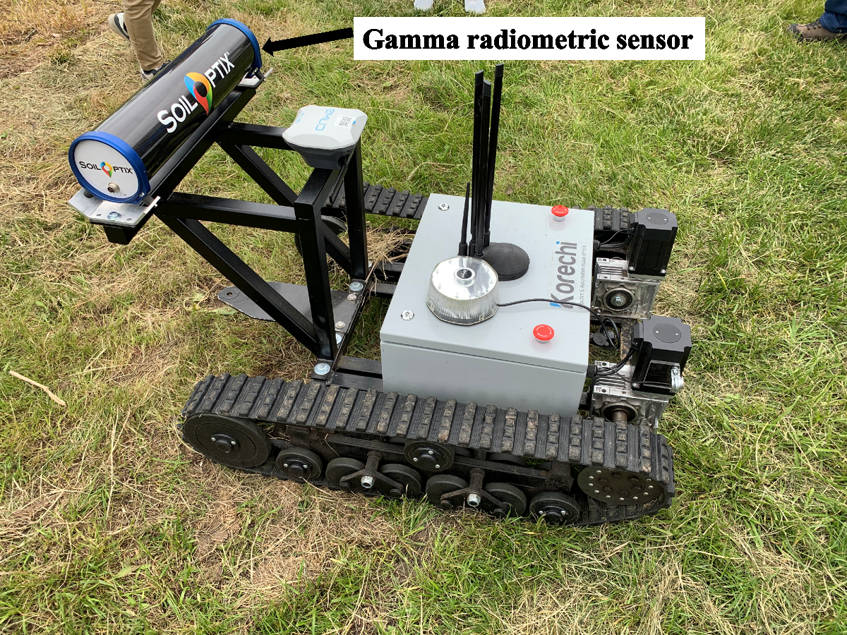
Figure 17.9. Remotely piloted aerial system (Sense-Fly eBee) that is equipped with a multispectral sensor (Sequoia Red-Edge). Photo credit: Ian Manning, Nova Scotia Community College – Centre of Geographic Sciences Applied Research. © Ian Manning. CC BY.

Proximal Soil Sensors: Whereas remote sensors are aerial- or space-based, proximal sensors are a suite of ground-based sensors that are designed to measure properties of soils that may be correlated to other soil properties. Given that measurements are taken on the ground, proximal soil sensors can characterize soil variability at a higher spatial resolution than remotely sensed data; and as a result, these sensors are more conducive for mapping soils at the field-scale. Figure 17.10 shows an unmanned ground vehicle that has been equipped with a gamma radiometric sensor system.

Amongst proximal soil sensors, electro-magnetic induction (EMI) sensors have been the workhorses for DSM and precision agriculture research (Doolittle and Brevik, 2014). The EMI sensor measures the apparent electrical conductivity (EC_a) of the soil at multiple depth intervals. Combined with a global positioning system (GPS), EMI survey data are often used as a predictor of soil properties such as soil salinity, clay content, and water content; however, secondary soil attributes, such as soil bulk density and soil organic carbon may also be derived from EC_a measurements. The EMI sensors are all but one type of proximal sensor—others may include gamma radiometric sensors, ground penetrating radar, and electrical resistivity sensors (amongst many). Interested readers are encouraged to refer to Viscarra Rossel et al. (2011) and Adamchuk et al. (2017) for a detailed overview of these systems.

Figure 17.10. Unmanned ground vehicle (Korechi) that is equipped with a gamma radiometric sensor (Medusa M1000). The vehicle has autonomous capability for navigation and can carry a variety of sensors. The gamma radiometric sensor pictured here collects data that can be related to soil physical and chemical properties, which can be mapped using information from the vehicle’s location. © Brandon Heung, Dalhousie University is licensed under a CC BY (Attribution) license.

Climate (c)

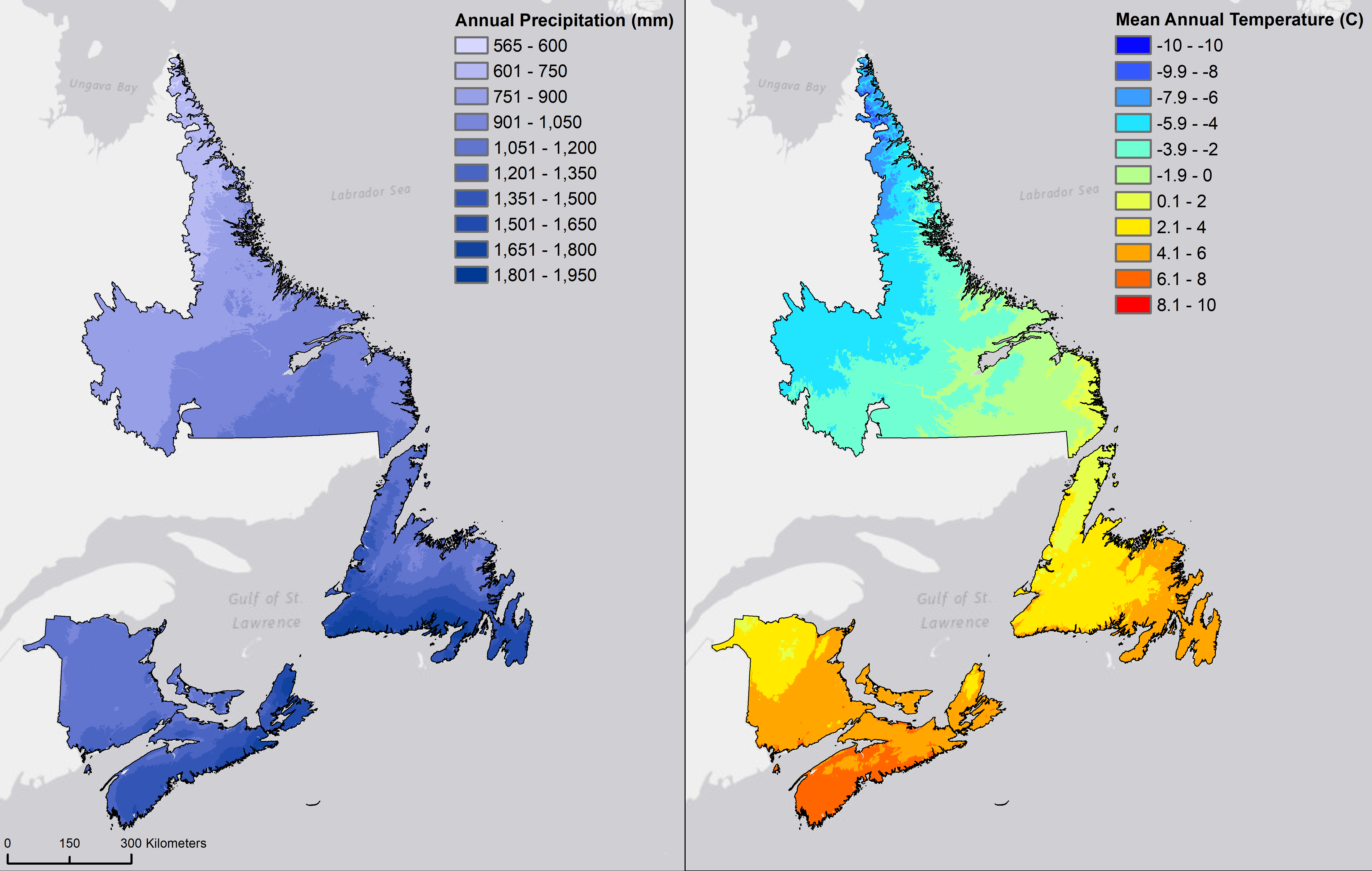
This factor is one of the least used scorpan factors (McBratney et al., 2003)—several possible explanations comes to mind. Firstly, the local climate is largely influenced by topography and as a result, topographic indices such as elevation and aspect may be used as a proxy for a climate variable due to the relationship between elevation and the environmental lapse-rate and the relationship between slope-face direction and temperature (Schaetzl and Anderson, 2005). However, as the extent of the study area increases to national- and global-scales, large-scale climatic patterns have been shown to be an important control on various soil properties—this was evident in the global SoilGrids250m product (Hengl et al., 2017). In terms of climate layers, common variables include mean annual temperature, mean annual precipitation, and evapotranspiration (McBratney et al., 2003). These datasets may be derived from sensors mounted on satellites; however, climate model data, often derived from weather stations, (e.g., WorldClim, ClimateNA) may also be used (Figure 17.11). In addition to using current climate conditions as inputs into a model, historical and projected future conditions could also be used to simulate the effects of changing climate conditions with respect to understanding the spatial and temporal patterns of soil properties.

Figure 17.11. Maps of mean annual precipitation and mean annual temperature for the Atlantic Provinces. Data set from the WorldClim version 2.0 at a 1 km spatial resolution (https://www.worldclim.org/). © Brandon Heung, Dalhousie University is licensed under a CC BY (Attribution) license.

Organisms (o)

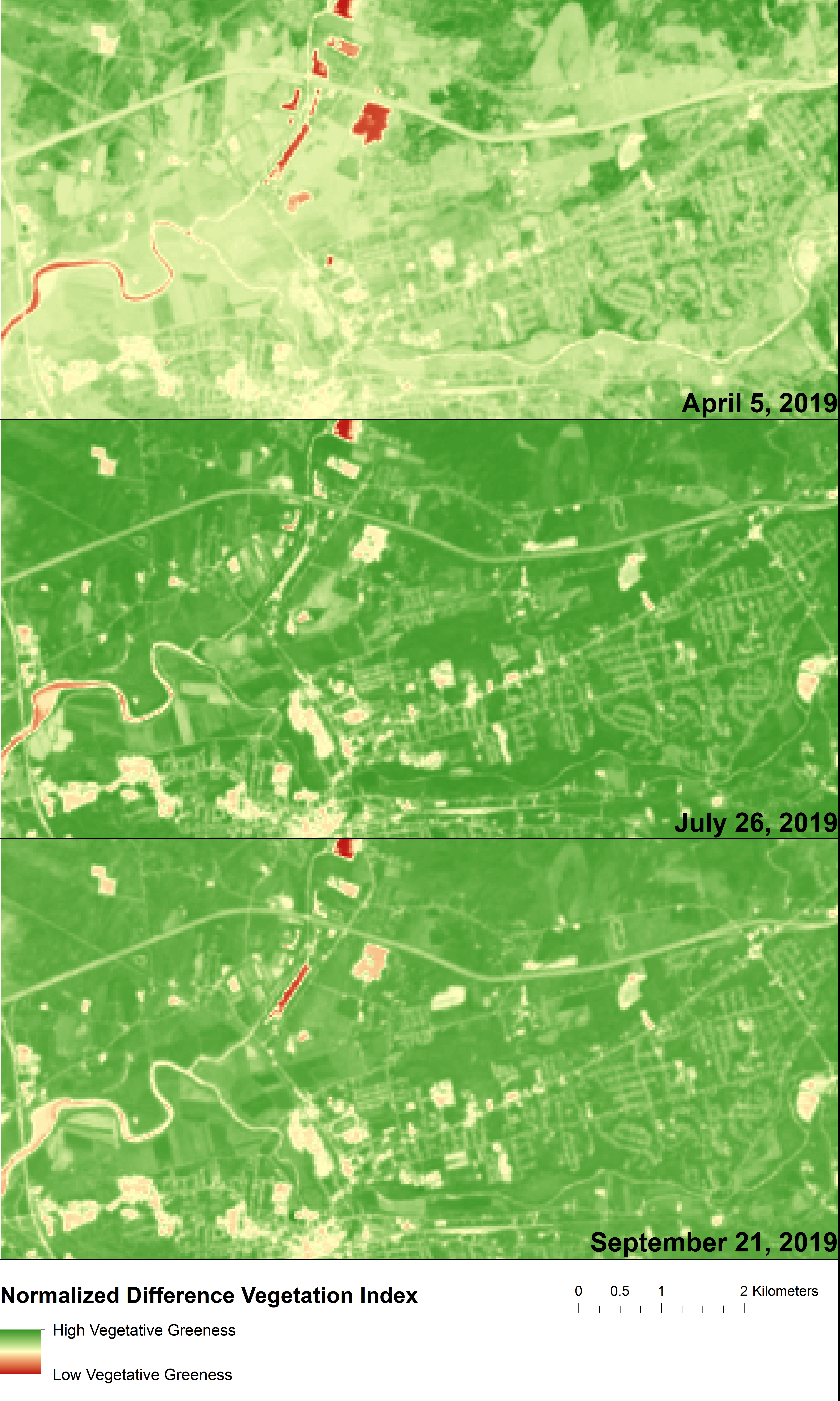
A major source of vegetation data used in DSM may be derived from satellite imagery where numerous vegetative indices have been developed based on satellite band-ratios (Mulder et al., 2011). Perhaps the most commonly used variable is the normalized difference vegetation index (NDVI), which provides a measure of vegetative greenness as a function of the near-infrared and red wavelengths from multispectral imagery. The NDVI and other remotely sensed data such as thermal imagery have also been shown to be an effective predictor for soil moisture, soil colour, soil texture, and water holding capacity; and it is also effective in evaluating plant growth (Figure 17.12; Mulder et al., 2011). In addition to NDVI, similar indices may include the Soil Adjusted Vegetation Index (SAVI), Transformed SAVI (TSAVI), Modified SAVI (MSAVI) and the Global Environment Monitoring Index (GEMI). Studies such as Paul et al. (2020) have found utility of these variables for mapping soil organic carbon and clay in the Lower Fraser Valley, BC; while Heung et al., (2017) used similar variables for mapping soil great groups for the Okanagan-Kamloops Region, BC. Similar indices may also be calculated using imagery that are acquired from a RPAS that is equipped with a multispectral or hyperspectral sensor. Although these indices have been extensively used in DSM, the data will be affected by the season and year from which the image was taken. If a soil mapper is requiring information on crop cover, imagery taken throughout the growing season would be more useful than post-harvest imagery.

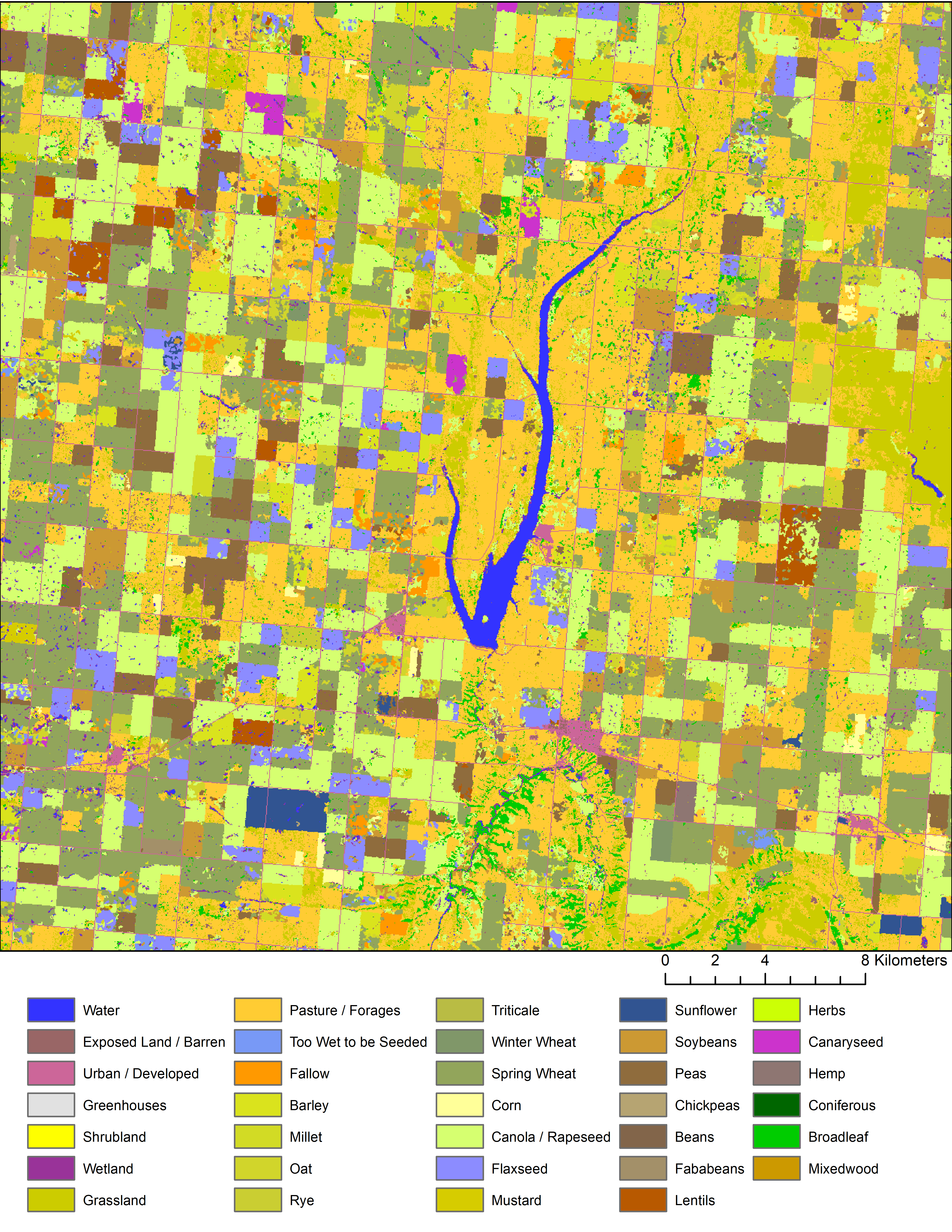
Figure 17.12. Normalized difference vegetation index maps produced from Landsat8 imagery for the Truro Region, Nova Scotia at a 30 m spatial resolution. © Siddhartho Paul, Post Doc with Heung, B. is licensed under a CC BY (Attribution) license.

In addition to using raw satellite imagery, researchers around the world have already processed vast quantities of imagery to generate landcover maps. For example, the North American Land Change Monitoring System provides landcover maps for 2005, 2010, and 2015 at a 30 m spatial resolution; and for a Canadian example, Agriculture and Agri-Food Canada have developed the Annual Crop Inventory data, which has been providing national-extent crop information since 2009 (Figure 17.13). However, it is necessary to recognize that these datasets are generated using predictive models; hence, it is important for a soil mapper to refer to the supporting documentation for these products and note their accuracy.

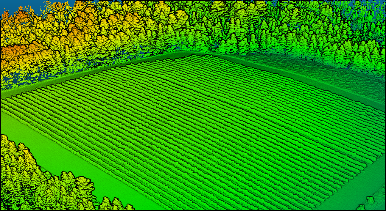
Figure 17.13. Annual Crop Inventory 2019 (Agriculture and Agri-Food Canada) for Moose Creek Region, Saskatchewan at a 30 m spatial resolution. © Brandon Heung, Dalhousie University is licensed under a CC BY (Attribution) license.

In other cases, crop data has also been used as a covariate for spatial prediction; for instance, crop yields are the result of the interaction between soils, plants, and atmosphere. Therefore, crop yield data may be used as an indicator for soil properties since plant growth is influenced by properties such as clay content, moisture content, and nutrient content for example (Shatar and McBratney, 1999; McBratney et al., 2000). In a forested setting, a possible opportunity may lie in the use of forest inventory data where forest variables such as basal area, gross total volume, stand density, stand height, and aboveground biomass might provide some insight into the soil properties. Especially with the developments in data acquired using light detection and ranging (LiDAR) technologies, forest inventory data might become more prevalent as a predictor (Woods et al., 2011; Treitz et al., 2012). Figure 17.14 shows a digital surface model that captures the variability in crop and tree height using LiDAR.

Figure 17.14. RPAS-acquired, LiDAR surface model for a vineyard in Middleton, NS. Image provided by Ian Manning, Nova Scotia Community College – Centre of Geographic Sciences Applied Research. © Ian Manning, Nova Scotia Community College – Centre of Geographic Sciences Applied Research is licensed under a CC BY (Attribution) license.

Relief (r)

It is well recognized that the r factor is the most used factor within DSM (McBratney et al., 2003). One of the staples in DSM research has been the use of a digital elevation model (DEM)—a raster that is made up of elevation values. DEMs may be produced from multiple sources: digitized contour maps; interpolated from ground measurements; and acquired from remote sensing using satellite- or RPAS-mounted sensors.

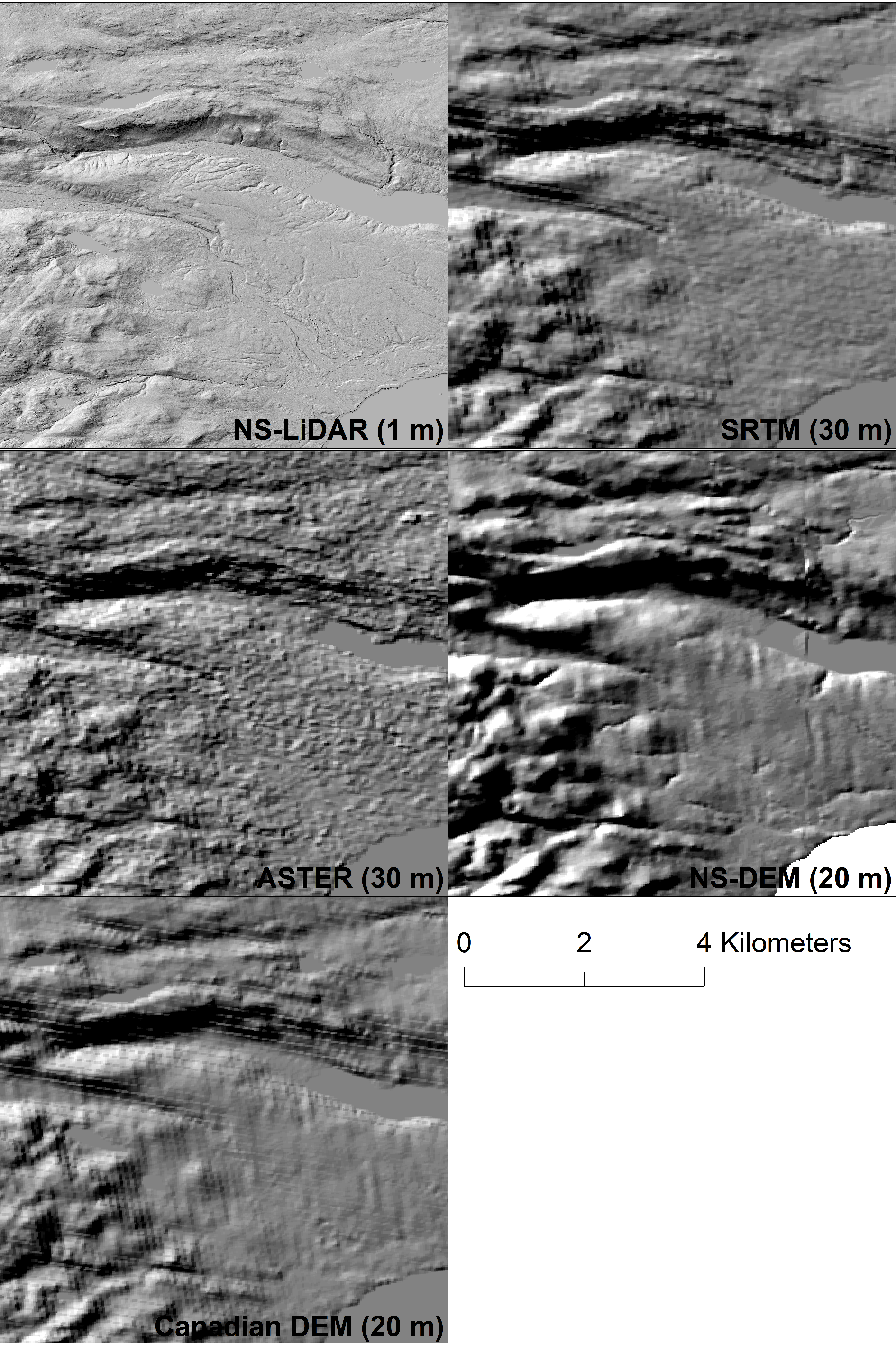
DEMs are particularly useful because they are readily available and typically free to access; for example, there are various provincial and federal DEM product(s) that are accessible via online web portals, and in parts of the country where there is no DEM data available, global DEM products such as Shuttle Radar Topography Mission (SRTM) or Advanced Spaceborne Thermal Emission and Reflection Radiometer (ASTER) may also be accessed. As a general recommendation, prior to using any DEM, it is always important for a soil mapper to visually assess the DEM by generating a hillshade (3D-like) representation of the topographic surface (Figure 17.15). This will help the mapper evaluate the abundance and types of DEM anomalies, due to the quality of the raw data, and the methods used to generate the DEM; and also whether preprocessing techniques (e.g., smoothing, pit filling, or road removal) should be applied.

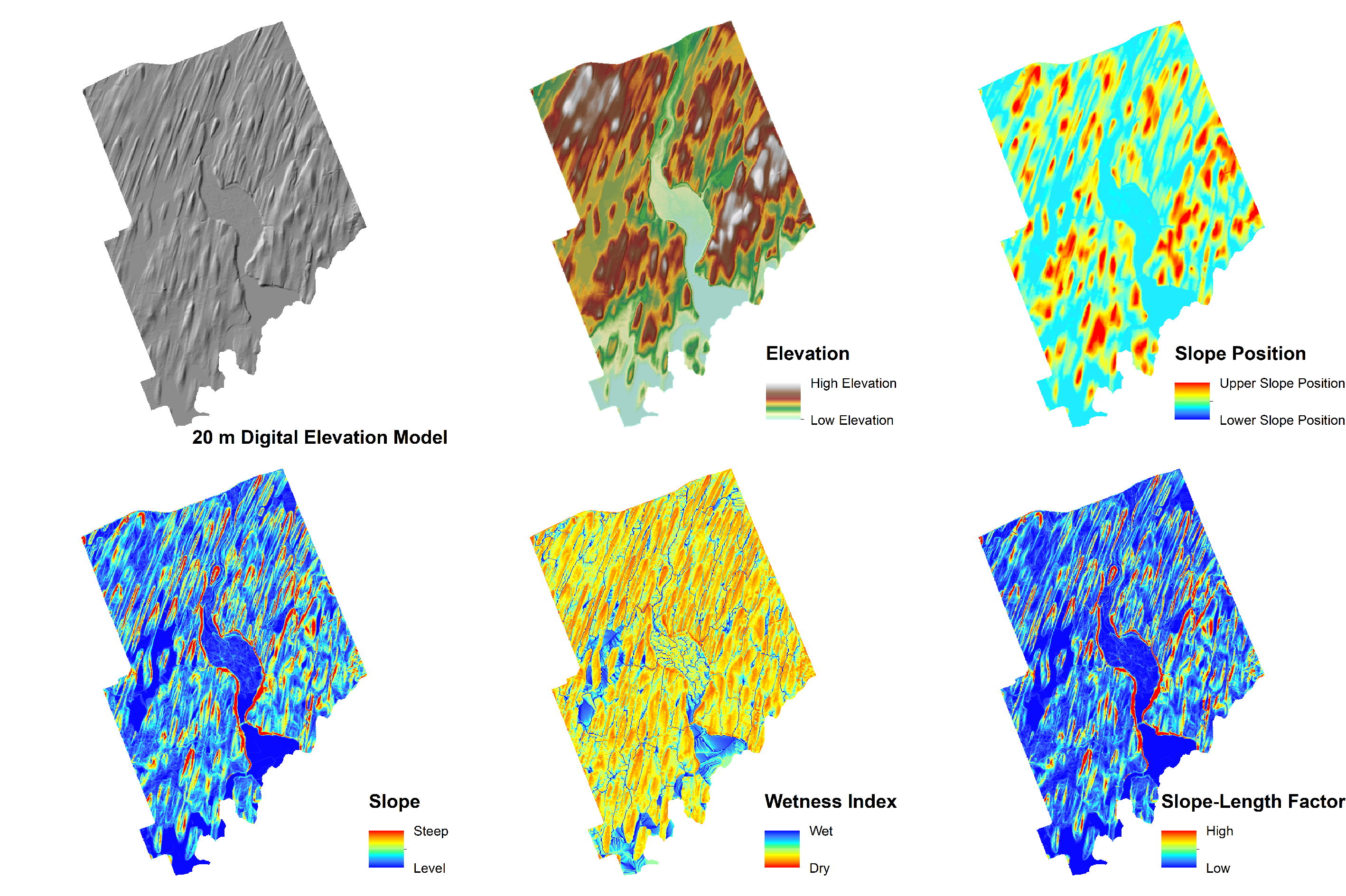
Figure 17.15. Comparison of hillshade models derived from Nova Scotia’s LiDAR data; Shuttle Radar Topographic Mission (SRTM) data; Advanced Spaceborne Thermal Emission and Reflection Radiometer (ASTER) data; Nova Scotia’s Enhanced DEM data; and the Canadian DEM data for a region west of Ingonish, Nova Scotia. © Brandon Heung, Dalhousie University is licensed under a CC BY (Attribution) license.

The value of a DEM comes from its flexibility in calculating a large suite of topographic variables. For example, a DEM can be used to characterize local-scale morphometry (e.g., slope, aspect, curvature), landscape-scale morphometry (e.g., relative slope position), and hydrological patterns (e.g., topographic wetness index) – all of which are influential on soil patterns (Figure 17.16). In fact, the analysis of land surface using various mathematical and statistical techniques, and the development of new topographic variables, are all part of the scientific discipline known as Geomorphometry.

Figure 17.16. Topographic variables derived from a 20 m digital elevation model for the Keene area, Ontario, at a 20 m spatial resolution. © Brandon Heung, Dalhousie University is licensed under a CC BY (Attribution) license.

Within Canada, high quality DEMs have been used as the basis for mapping soil parent materials (Heung et al., 2014), soil types (Heung et al., 2016), and soil thickness (Scarpone et al., 2016) throughout BC; and mapping soil depth and textural classes throughout ON (Akumu et al., 2015; Akumu et al., 2016). In fact, those studies generally used only DEM-derived data.

Furthermore, the topographic variables may also be used to delineate landform features (Figure 17.17). In Pennock et al. (1987), combinations of planform (change in aspect) and profile curvature (change in slope) were classified into a series of seven landform elements (i.e., divergent/convergent shoulders; divergent/convergent backslopes; divergent/convergent footslopes; and level surfaces) that characterized the topographic controls on the flow of sediment and water. As a result, similar landscape classification schemes could be applied using a DEM (e.g., MacMillan et al., 2000, 2004) in a semi-automated approach.

Figure 17.17. 3-dimensional representation of a landform classification map produced using a 25 m spatial resolution DEM for the Twin Sisters watershed, British Columbia. © Brandon Heung, Dalhousie University is licensed under a CC BY (Attribution) license.

Parent Material (p)

Information on soil parent materials have typically been acquired from digitized geological maps; hence, they share similar spatial problems to conventional soil survey maps whereby there may be a combination of complex map units; the amount of detail is controlled by the mapping scale; and detailed maps may be limited in coverage. As a result, soil parent material is an attribute of the soil that has previously been mapped using predictive approaches; for example, Heung et al. (2014) produced a parent material map for the Lower Fraser Valley, BC.

When using digitized geological maps, it is important to recognize the source of material from which the soil is derived (Figure 17.18). For example, a bedrock geology map would likely find greater use in non-glaciated environments where the soil is largely derived from weathered bedrock. However, Canadian landscapes are predominantly glaciated and therefore the overlaying sediment may have contrasting properties to the bedrock and hence, a surficial geology map would be more useful as it characterizes the material that has been transported and deposited on the bedrock. These mapping efforts have highlighted the close associate between topography and parent material, particularly in glaciated environments, so combinations of topography derivatives are often used in DSM as a surrogate for parent material.

Figure 17.18. Maps of bedrock geology (left) and surficial geology (right) for the Atlantic provinces. The bedrock geology data are from the Geological Map of Canada (Wheeler et al., 1997) and the surficial geology map is derived from the Surficial Materials Map of Canada data set (Fulton, 1995). © Brandon Heung, Dalhousie University is licensed under a CC BY (Attribution) license.

Age (a)

The age factor may be used to describe how long pedogenesis has occurred and may be estimated as the age of the ground or material from which the soil has developed (McBratney et al., 2003). Within DSM, there are very few examples where this information has been used due to the difficulty in characterizing the age of soil within a format that would be conducive for use within a GIS. One potential option for incorporating the a factor into a DSM framework would be by incorporating information on how humans have modified the landscape and thereby influencing soil attributes and types.

Spatial Position (n)

The n factor may be incorporated in several ways: using the spatial coordinates of soil sample locations or using a raster layer that represents the distance to some geographical phenomenon.

Spatial Coordinates of Soil Samples: Predicting soil attributes may be carried out by using only the spatial coordinates of the soil samples themselves. Here, we should introduce Waldo Tobler’s First Law of Geography (Tobler, 1970), which states:

“Everything is related to everything else, but near things are more related than distant things.”

When applied to DSM, we can therefore say that two soil samples that are in close proximity are more likely to share similar soil properties than two soil samples that are located far from each other. As a result, the relationship between the sampling location, its corresponding soil value, and its distance to neighboring sampling locations can be used to predict (i.e., interpolate) soil values between those locations using geostatistical approaches. Although an overview of geostatistics is far beyond the scope of this textbook, students that have taken a spatial analysis class would be familiar with interpolators such as inverse distance weighting and kriging approaches.

Within Canada, geostatistical approaches have been used to characterize soil variability as early as the 1980’s. In Raymond, Alberta, Chang et al. (1988) established a grid of 64 sampling points over a 20 × 25 m agricultural field to map sand content and soil salinity using kriging to facilitate irrigation practices on saline soils. Within a forested system located in southwestern BC, Chandler et al. (2008) applied a similar approach using gridded sampling and kriging to evaluate the localized, spatial patterns of forest floor nutrients as influenced by a bigleaf maple tree within a conifer-dominant stand.

Distance-Based Raster: Information on spatial position may also be incorporated by calculating the distance or proximity of each pixel within the study area to certain geographical phenomenon, or reference point, to capture contextual information about the landscape. For example, using a stream network, a distance-to-nearest-stream layer may be calculated; furthermore, similar distance-based layers may be calculated to represent the proximity to the ocean, lakes, rivers, geomorphic features, and many other features. Studies such as Heung et al. (2014) have found that when mapping soil parent materials for the Lower Fraser Valley, BC, layers representing the distance to the nearest stream and to the Fraser River were important for predicting the distribution of fluvial materials.

Soil Sampling

The foundation of soil survey rests upon selection of representative sampling sites. With fewer resources available to complete large field programs and recent advances in computational tools, new techniques to optimize sample site selection are being used to improve accuracy of predictive models while gaining efficiencies in field sampling. Soil sampling in DSM seeks to gather information to understand the development and distribution of soils as expressed by soil forming factors (Jenny, 1941), or the scorpan model variables (McBratney et al., 2003). At its most basic, the sampling design seeks to sample representatively from the geographic area of interest and all the soil forming factors (i.e., covariates); the underlying assumption is that the spatial variability of soil properties being predicted can be explained by the environmental covariates.

There are many approaches to sampling design, including statistical and geometric approaches that seek to select samples randomly from all possible sampling locations (population) or distribute sample locations in geographic space based on spatial position or coordinates, and approaches that use ancillary data to select sample locations, commonly referred to as feature space approaches.

At the heart of every sampling program is the question of what attributes to measure at each field location. This question is closely related to a problem that was common for conventional soil mapping, namely the development of the map legend. Depending on the level of detail desired in the final product, and available survey resources, the need for agglomeration and subdivision of soil classes, the depth requirements for soil property evaluation, and the specific methods for field sampling and analysis all affect the final map, and the types of information in the training dataset. Ultimately, these considerations must support the original objectives set out for the DSM project.

The most commonly used geometric approaches include grid sampling (GS), simple random sampling (SRS), stratified random sampling (StRS), transect sampling (TS), cluster sampling (CS) and nested sampling (NS). Grid sampling divides the study area into an evenly-spaced regular grid with sample locations at the centre of each grid; the grid size is specified by the user based on some criteria, usually time, budget or prior knowledge of the required sampling density. Simple random sampling creates sampling sites that are selected completely at random (Brus et al., 2011) from the available study area with equal probability of being selected (Biswas and Zhang, 2018). Stratified random sampling is similar to SRS with the exception that the area is subdivided into smaller blocks, called strata, and SRS is applied to the strata (Brus and de Gruijter, 1997). The size of the strata can be used to weight the sampling, resulting in proportional sampling of the strata (Pennock and Yates, 2007). Transect sampling is a form of cluster sampling where samples are selected at equal distance intervals along a line (de Gruijter and Marsman, 1985). In cluster sampling, sample locations are grouped closely, a technique used to enable sampling in rough terrain with inaccessible areas without compromising accuracy (Biswas and Zhang, 2018). Nested sampling is typically applied in combination with other sampling designs and quantifies the variability of the data along different distances, a concept originating from geostatistics. Examples of sample designs are provided in Figure 17.19.

Figure 17.19. Examples of three sampling designs. Small black dots represent sampled raster cells. Shown are simple random sampling (left), stratified random sampling (middle) where colors (green, yellow and white) indicate a theoretical stratification in the data into three levels, and chessboard-style grid sampling (right). © Daniel D. Saurette, Ontario Ministry of Agriculture, Food and Rural Affairs is licensed under a CC BY (Attribution) license.

Feature space approaches consider the values of environmental covariates at the sampling locations. Fuzzy k-means sampling (FKMS) uses the k-means clustering algorithm to minimize the distance between sampling locations, but this distance is in covariate space, not geographic space (Brus, 2019). The conditioned Latin hypercube sampling (cLHS) was proposed by (Minasny and McBratney, 2006) as a modification to Latin hypercube sampling (Mckay et al., 1979). With many covariates, a full factorial experiment is unfeasible—the Latin hypercube sampling allows sampling of all covariates, with one sample per strata (Brus, 2019).

An optimal sampling design should provide adequate coverage of both geographic and feature space. This can be assessed using various tools. For feature space coverage, typically a comparison of the feature space coverage of the sample sites and that of the entire study area can be completed to determine the adequacy of the sampling design. Tools exist to optimize sampling in terms of geographic space and in terms of feature space, however the fusion of these two sample optimization strategies remains an important area of research. One aspect lacking from existing sampling strategies is information regarding the optimal number of sites required to optimize the predictive ability of a model used for DSM. Interested readers are encouraged to refer to Brus et al. (2011) and Biswas and Zhang (2018) for a more detailed introduction to sampling design.

Sampling design and soil sampling present many technical and logistic challenges. During the sampling design phase, the soil mapper must consider features that are to be avoided during sample selection, especially given the use of computer algorithms, which cannot recognize these restrictions when selecting sample sites. For example, anthropogenic features such as roads, buildings, quarries, and natural features such as water bodies, are typically of little interest for soil mappers and should be removed from the layers of information used to design the sample plan. Similarly, in difficult terrain or remote areas, one might choose to restrict the sample selection process to a manageable buffer distance from access roads. Access to private lands for soil sampling can be challenging. Restricting the sampling design to public lands is in most cases impractical and not feasible, and as such permission from landowners must be acquired to complete soil sampling field work. A common issue that arises is the need for an alternate sampling site when access to private land is denied. Although beyond the scope of this introduction to DSM, researchers are developing strategies to modify and adapt sample design algorithms to account for these types of restrictions (Clifford et al., 2014; Malone et al., 2019).

Prediction of Soil Classes and Properties

Developing a soil map using DSM techniques largely requires the following three ingredients:

a suite of environmental layers (i.e., predictors or covariates) that represent the scorpan factors;
soil data that are geospatially referenced; and
a model that characterizes the relationship between the soil data and the environment in order to make predictions for unsampled locations.

In the previous sections, we have explored the different sources of environmental data and described the various spatial sampling approaches used to acquire the soil data. In this section we describe the process required to create a training dataset, which is then used to calibrate a predictive model to generate map outputs.

Typically, DSM techniques involve a form of supervised learning where a training dataset is first created by spatially intersecting the sample locations (with measured soil properties) with the underlying suite of environmental layers. Using a predictive model, the relationship between the soil response variable and the environmental predictor layers is established using a classification or regression function (i.e., model fitting). Once the predictive model is fitted with the training data, it is then applied to the set environmental layers to predict the soil properties or classes at unsampled locations.

Prior to making predictions, the soil mapper must recognize the type of soil data that is to be predicted. Soil data may take the form of categorical data or continuous data, whereby categorical data may be further subdivided into nominal data and ordinal data. Nominal data describe the qualitative aspects of soil and have no quantitative value and the most common example of nominal data would be the soil’s taxonomic unit (e.g., soil order, great group, series) but may also include soil parent material class, soil textural class, and others. Ordinal data, another type of categorical data, represent values that have ordered units (i.e., values are relative to each other), where examples may include soil moisture and nutrient regime classes. With soil moisture regime, there are nine potential values ranging from 0 to 8, where a value of 0 represents ‘very xeric’ conditions while a value of 8 represents ‘hydric’ conditions; however, the exact difference between the values are not known. In contrast, continuous data represents measured soil properties such as soil depth, soil pH, clay content, soil organic carbon stock, and many more.

The distinction between categorical and continuous data types when representing soil information is critical because it largely determines which predictive model and methods for assessing model accuracy and uncertainty are appropriate. When predicting categorical soil data, we are limited to the use of predictive approaches that are suitable for classification purposes, whereas, the prediction of continuous data requires the use of regression modelling approaches. An example of a digital soil map produced using a regression modelling approach is shown in Figure 17.6 (right) for soil organic carbon predictions and an example using a classification modelling approach is shown in Figure 17.20 for soil great group.

Figure 17.20. Soil great group map of the Lower Fraser Valley, British Columbia using support vector machine with radial basis function classifier at a 100 spatial resolution with a 72% overall accuracy. © Brandon Heung. CC BY.

A comprehensive overview of the modelling approaches is far beyond the scope of this textbook; however, interested readers should refer to McBratney et al. (2003), which provides an overview of various modelling approaches for regression and classification using machine-learning and geostatistical techniques. For a detailed overview of machine-learning techniques used for classification purposes in DSM, readers may refer to Heung et al. (2016).

It is important for readers to realize that there are many different types of predictive modelling techniques that are used in DSM, as well as in disciplines beyond DSM; however, there is not a single model that will consistently outperform another or is considered to be “best” in all situations. The choice in environmental predictor layers, the nature of the soil-environmental relationships (e.g., linear vs. non-linear relationships), the size of the training dataset, soil property, as well as a whole host of other factors, may affect a model’s performance. Furthermore, the intrinsic properties of the model, such as processing time, computational demand, and model complexity, will vary. As a result, it is encouraged that DSM practitioners compare a variety of modelling techniques and perform an accuracy assessment of all results; furthermore, a visual assessment of the mapping outputs should be carried out by a trained soil scientist to ensure that the soil maps are consistent with a pedological understanding of the landscape.

Given that much of the modelling process may be carried out in an automated way using statistical software such as R, the automation greatly facilitates model comparisons and the process of comparing models should be considered as ‘best practice’. For example, in Heung et al. (2016), identical input data were used to train 11 modelling techniques, where it was determined that despite the same inputs, the model outputs varied drastically when mapping soil great groups for the Lower Fraser Valley, BC (Figure 17.21).

Figure 17.21. Close-up maps of soil great group predictions for the Lower Fraser Valley at a 100 m spatial resolution using a variety of classification algorithms. All predictions were generated using the same set of input data. Predictive models include (A) CART with bagging, (B) CART, (C) k-nearest neighbours, (D) logistic model tree, (E) multinomial logistic regression, (F) artificial neural network, (G) nearest shrunken centroid, (H) Random Forest, (I) linear support vector machine, and (J) support vector machine with radial basis function. © Brandon Heung. CC BY.

Accuracy Assessment

All maps approximate reality and all digital soil maps will deviate from the real world and whatever is generated from the model is only one out of an infinite number of realizations of a soil map. Again, this is demonstrated in Figure 17.21, which shows that different models could generate drastically different realizations of a soil map. Therefore, to quantify the quality of map predictions, an accuracy assessment needs to be carried out on all predictions. Here, we describe the term ‘accuracy’ as being the difference between the observed and predicted values at a location (Brus et al., 2011); whereby we can describe the accuracy as being ‘higher’ as the difference decreases.

Similar to selecting the appropriate model type to predict categorical and continuous soil variables, the choice of appropriate accuracy metrics also depends on this. However, in both cases, accuracy assessment must be carried out using an independent (i.e., validation or test) dataset that was not used to train the model.

When assessing the accuracy of categorical predictions (e.g., soil series, soil parent material type), we generally rely on overall accuracy and Cohen’s kappa coefficient as the main metrics. The overall accuracy is the proportion of observations that were correctly predicted for the independent dataset; whereas kappa accounts for the by-chance agreement between the observed and predicted classes. Both metrics range from 0 to 1, where a value of 1 represents high accuracy.

When assessing the accuracy of continuous predictions (e.g. bulk density, soil organic carbon), the mean square error (MSE), root mean square error (RMSE), coefficient of determination (R²), and Lin’s concordance correlation coefficient (CCC) are often used. The MSE is effectively the average squared difference between the observed and predicted values; in comparison, the RMSE, is the square root of MSE and is expressed in the same units as the soil variable. In both cases, a lower MSE or RMSE represents a more accurate model. R² measures how closely the observed and predicted values follow along a best-fit regression line (i.e., how closely the values are correlated) and represents the proportion of soil variation that is explained by the model. It is critical to note that R² does not represent accuracy because it does not account for model bias whereby the model may consistently overpredict or underpredict a soil variable. Instead, the more appropriate metric is to use CCC, which represents the goodness of fit along a 45° line on a scatterplot of observed and predicted values. Values of CCC range from 0 to 1, where values of 1 represent scenarios where the predicted values match the observed values and thus indicates high prediction accuracy and precision.

UNCERTAINTY IN DIGITAL SOIL MAPS

It is important to recognize that along with all environmental modelling activities, models are simply abstract representations of the real world and that there are uncertainties about the true properties of the soil. How we present soil patterns on a soil map is based on a predictive model, which is never truly free of errors; hence, quantitatively estimating the uncertainty of digital soil maps is just as important as validating it because it will allow users to assess the usefulness of the maps and how those maps may be used (Heuvelink, 1998). Uncertainties are accumulated and propagated from three sources: the measured soil property, the environmental predictors representing the scorpan factors, and the predictive model.

Uncertainty in Soil Properties: Whenever a soil sample is taken to a lab, there will always be differences in analytical techniques that may contribute errors when measuring various soil properties. In some situations, the soil response variables may be inferred from other soil variables that are easier to measure using pedotransfer functions whereby errors may be further propagated. Uncertainties could also arise when recording the spatial location of sample points when using a GPS, whereby some GPSs are more accurate than others.

Uncertainty in Environmental Predictors: There is inherent uncertainty with environmental predictors themselves. For example, vertical uncertainties may be present with DEMs as well as measurement uncertainty from remote and proximal soil sensors. When using conventional soil maps or geology maps in the polygon format, the composition of the polygon, polygon boundaries, and map scale may all contribute to uncertainty.

Uncertainty in Predictive Model: As previously discussed, the choice of predictive model may result in drastically different soil maps; and hence, the structure of the model may be another source of uncertainty. The relationships between the environmental predictors and soil properties may be linear, non-linear, or a combination of both, and certain types of models are more effective at capturing those relationships than others. For examples, a simple linear model would be effective at modeling linear relationships, whereas non-linear modelling approaches (e.g., classification and regression trees) are effective at capturing the non-linear, hierarchical relationships. Finally, some modelling approaches (e.g., model trees) are a hybrid of linear and non-linear models and are therefore able to capture both types of relationships.

Ideally, all digital soil maps should be accompanied with uncertainty maps, which estimate the uncertainty for each individual pixel—in practice, however, this is often not the case. Due to the importance of recognizing uncertainty in model outputs, international mapping standards (e.g., GlobalSoilMap.net) often require the inclusion of a 90% prediction interval map as well as the lower (5%) and upper (95%) prediction limits (Figure 17.22). Here, we assume that with a 90% confidence level, the real value of a soil property will be within the prediction interval. Therefore, when interpreting these uncertainty maps, the uncertainty will increase as the 90% prediction interval width increases. It should be noted that this representation of uncertainty only applies to continuous soil variables.

Figure 17.22. Series of maps used to represent uncertainty of digital soil mapping of soil pH in Ottawa, Ontario: prediction, prediction interval width (90%), and the lower (5%) and upper (95%) prediction limits. © Daniel D. Saurette, Ontario Ministry of Agriculture, Food and Rural Affairs is licensed under a CC BY (Attribution) license.

When representing uncertainty for predictions of categorical soil variables, class probability maps are used to calculate uncertainty for each pixel. Here, a set of probability rasters are produced for each class, whereby each pixel has a corresponding value that represents the probability of that class occurring (Figure 17.23). If an individual class has a high probability of occurrence, the uncertainty is low; however, if all the classes have an equal probability of occurrence, the uncertainty is high. Although there are many metrics that may be calculated from these class probability rasters (e.g., ignorance uncertainty, exaggeration uncertainty, confusion index), they are all effectively characterizing the spread in probability values amongst the various classes (Figure 17.24).

Figure 17.23. Class probability maps for soil great group prediction for the Okanagan-Kamloops region of British Columbia derived at a 100 m spatial resolution using the Random Forest classifier. Most frequently occurring soil great groups include Humo-Ferric Podzols (HFP), Gray Luvisols (GL), Dystric Brunisols (DYB), Eutric Brunisols (EB), and Black Chernozems (BLC). © Brandon Heung. CC BY.

Figure 17.24. Ignorance uncertainty map produced from the soil great group probability maps at a 100 m spatial resolution for the Okanagan-Kamloops region of British Columbia. Higher values (red) represent higher uncertainty. © Brandon Heung, Dalhousie University is licensed under a CC BY (Attribution) license.

BEYOND DIGITAL SOIL MAPPING

Much effort has been made in improving the accessibility, interpretability, understanding, and communication of soil information to data users in some provinces. Online applications, such as the British Columbia Soil Information Finder Tool (SIFT), Agricultural Land Resource Atlas of Alberta, the Saskatchewan Soil Information System (SKSIS), Info-Sols (Québec) and the Ontario Agricultural Information Atlas, leverage legacy soil maps and provide a graphical user interface whereby a user could easily query those maps and acquire information related to soil properties as well as interpreted soil information including agricultural land capability and soil erosion risk.

Other platforms, such as SOILx, have explored the use of augmented reality in visualizing soil profiles on a mobile device. These platforms have the potential to improve decision-making processes, aid environmental impact assessments, and provide sustainable soil management information to users. However, these platforms are limited by the quality of the soil information that populates them and the user’s ability to understand that information.

Traditionally, soil mappers have focused on the development of quantitative methods for predicting the soils over space. However, the other critical role of a soil mapper, which has received far less attention, is that of a “knowledge generator and provider” and understanding how soil information may be used to inform decision-making and resource-planning practices (Finke, 2012). Together with domain-experts (e.g., agronomists, foresters, environmental scientists, engineers), the role of the soil mapper is to collectively interpret the various digital soil maps and develop interpretive tools that assess soil threats and functions and facilitate the decision-making process. For example, a soil erosion risk map is probably more useful to a decision-maker than individual maps of soil properties (e.g., organic matter and soil texture maps) and other environmental data layers (e.g., slope and rainfall maps).

Within the pedometrics community, a large part of the discipline is devoted to using digital soil maps as ingredients for assessing soil functions and threats. This active area of research is referred to as digital soil assessments (DSA). While the details of DSA is beyond the scope of this chapter, interested readers should refer to Carré et al. (2007), who first introduces this field, and Finke (2012), who subsequently discusses the scope of the field. Globally, there has been tremendous progress towards developing soil assessment tools using digital soil maps.

Applications of digital soil information

Applications may include, but are not limited to:

Mapping management zones for variable rate fertilizer and irrigation applications (Fleming et al., 2000)
Assessing regional-scale agricultural land suitability (Harms et al., 2015; Kidd et al., 2015)
Estimating the potential gross margins for specific crops (Kidd et al., 2015)
Evaluating national-scale soil erosion (Panagos et al., 2015)
Assessing soil carbon sequestration potential (Angers et al., 2011; Akpa et al., 2016)
Aiding the provision of site- and soil-specific insurance to manage soil threats (Cook et al., 2008)
Assessing human exposure to soil contaminants (Caudeville et al., 2012)
Characterizing wine regions (terrons and terroir) using climate and soil information (Carré et al., 2005; Coggins et al., 2019)
Developing ecosite maps for stand-level forest management plans (Yang et al., 2017)
Mapping landscape-scale soil health indices (Svoray et al., 2015)
Farm-scale soil organic carbon audits and monitoring (de Gruijter et al., 2016; Malone et al., 2018)

Can You Dig It!

The Canadian Digital Soil Mapping Working Group

Canadian-digital-soil-mapping-working-group-e1619330518938.png — **(Top)** First meeting of the CDSMWG held in 2016, Quebec City; **(Middle)** First education workshop on digital soil mapping held at Simon Fraser University, 2017, and in Vancouver, BC; **(Bottom)** Members of the CDSMWG at the Canadian Society of Soil Science Annual Meeting, 2019 held at University of Saskatchewan, Saskatoon, SK. © Soils of Canada website (https://soilsofcanada.ca/digital-soil-mapping); Brandon Heung, Dalhousie University is licensed under a CC BY (Attribution) license.

Over the last 20 years, the soil science community has evolved from the dominance of government soil surveyors and university scientists to a community where scientists with soil expertise are working in every public and private sector (e.g. agriculture, forestry, environment) and across Canada’s diverse landscape. Unfortunately, this has led to the decentralization and dispersion of soil information and soil mapping expertise.

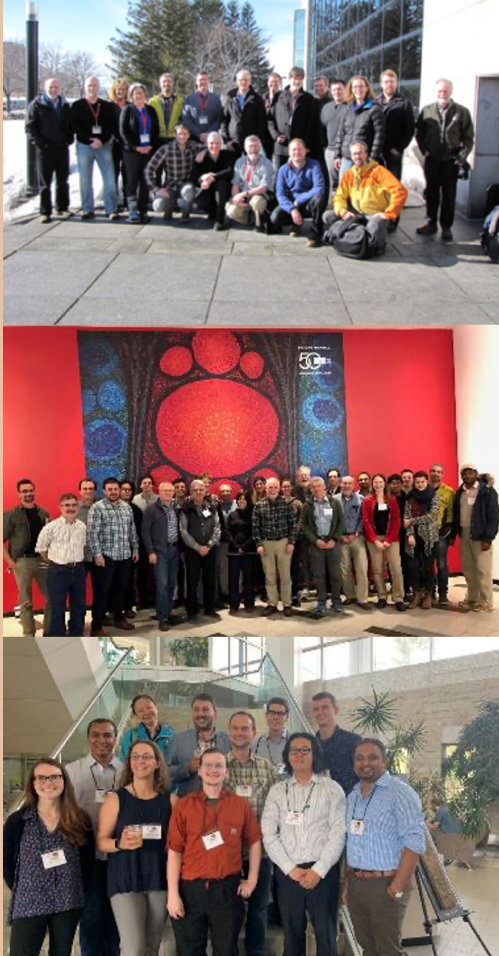
Out of that recognition, a major development in the national soil mapping landscape was the establishment of the Canadian Digital Soil Mapping Working Group (CDSMWG)—a national scientific network with researchers from multiple academic institutions, federal government departments, and provincial agencies. To provide a mechanism and platform for soil mappers to collaborate at the national-scale, the Pedology Committee of the Canadian Society of Soil Science (CSSS) established the CDSMWG in 2016. This cross-country, cross-sector research network is tasked with coordinating national-scale DSM initiatives, disseminating digital soil information, and delivering educational workshops.

For example, the community developed the soil carbon maps of Canada for submission to the FAO’s global carbon mapping project. All products developed by the CDSMWG are designed to meet international DSM standards of GlobalSoilMap.net and the Food and Agriculture Organization (FAO) of the United Nations. To date, the CDSMWG has been successful in its mandate; it was instrumental in developing and delivering a preliminary Canadian Soil Organic Carbon Map (CSOC map) as part of Canada’s contribution to the Global Soil Organic Carbon Map (GSOC map) compiled by the Intergovernmental Technical Panel on Soils of the FAO in 2017 (FAO and Intergovernmental Technical Panel on Soils, 2018). Dedicated volunteers in the project clearly demonstrated the network’s ability to effectively communicate and collaborate in the daunting task of developing the CSOC map.

In addition, members of the CDSMWG are also dedicated to training the next generation of digital soil mappers and have offered multiple workshops across the country thus far. Workshop attendees have included undergraduate and graduate students, university and government researchers, and industry participants.

THOUGHT EXERCISES

Brainstorm some ways on how digital soil maps may be used for addressing environmental and resource management issues at local-scales (e.g., individual farm fields or forest stands), regional-scales (e.g., individual provinces), and national-scales (e.g., Canada).

Digital soil data is becoming increasingly available in Canada. Please take some time to explore the following resources and brainstorm the benefits and challenges of digital soil mapping: British Columbia Soil Information Finder Tool; Saskatchewan Soil Information System; and Ontario AgMaps Geographic Information Portal. International resources available include: Australian Soil Resource Information System, and SoilGrids.

REFERENCES

Adamchuk, V., Allred, B., Doolittle, J., Grote, K., and Viscarra Rossel, R. 2017. Chapter 6: Tools for proximal soil sensing. In Soil Survey Manual, Soil Science Division Staff. Agricultural Handbook No. 18, United States Department of Agriculture, pp. 355-394.

Angers, D.A., Arrouays, D., Saby, N.P.A., and Walter C. 2011. Estimating and mapping the carbon saturation deficit of French agricultural topsoils. Soil Use Manage. 27: 448-452.

Akpa, S.I.C., Odeh, I.O.A., Bishop, T.F.A., Hartemink, A.E., and Amapu, I.Y. 2016. Total soil organic carbon and carbon sequestration potential in Nigeria. Geoderma 271: 202-215.

Akumu, C.E., Johnson, J.A., Ethreidge, D., Uhlig, P., Woods, M., Pitt, D.G., and McMurray, S. 2015. GIS-fuzzy logic based approach in modeling soil texture: Using parts of the Clay Belt and Hornepayne region in Ontario Canada as a case study. Geoderma 239-240: 13-24.

Akumu, C.E., Woods, M., Johnson, J.A., Pitt, D.G., Uhlig, P., and McMurray, S. 2016. GIS-fuzzy logic technique in modeling soil depth classes: Using parts of the Clay Belt and Hornepayne region in Ontario, Canada as a case study. Geoderma 283: 78-87.

Arrouays, D., Grundy, M.G., Hartemink, A.E., Hempel, J.W., Heuvelink, G.B.M., Hong, S.Y., Lagacherie, P., Lelyk, G., McBratney, A.B., McKenzie, N.J., Mendonça -Santos, M.L., Minasny, B., Montanarella, L., Odeh, I.O.A., Sanchez, P.A., Thompson, J.A., and Zhang, G-L., 2014. GlobalSoilMap: Toward a fine-resolution global grid of soil properties. Adv. Agron. 125: 93-134.

Beckett, P.H.T. 1971. The cost-effectiveness of soil survey. Outlook Agr. 6: 191-198.

Bie, S.W., Ulph, A., and Beckett, P.H.T. 1973. Calculating the economic benefits of soil survey. J. Soil Sci. 24: 429-435.

Biswas, A., and Zhang, Y. 2018. Sampling Designs for Validating Digital Soil Maps: A Review. Pedosphere 28: 1–15.

Brus, D.J., and de Gruijter, J.J. 1997. Random sampling or geostatistical modelling? Choosing between design-based and model-based sampling strategies for soil (with discussion). Geoderma 80: 1–44.

Brus, D.J., Kempen, B., and Heuvelink, G.B.M. 2011. Sampling for validation of digital soil maps. Eur. J. Soil Sci. 62: 394-407.

Brus, D.J. 2019. Sampling for digital soil mapping: A tutorial supported by R scripts. Geoderma 338: 464–480.

Canada Soil Survey Committee, 1978. The Canadian System of Soil Classification. 1st ed. Research Branch, Canadian Department of Agriculture.

Carré, F., and McBratney, A.B. 2005. Digital terron mapping. Geoderma 128: 340-353.

Carré, F., McBratney, A.B., Mayr, T., and Montanarella, L. 2007. Digital soil assessments: Beyond DSM. Geoderma 142: 69-79.

Caudeville, J., Goovaerts, P., Carré, F., Bonnard, R., Arrouays, D., Cicolella, A., Jolivet, C.C., Saby, N.P.A., and Boudet, C. 2012. Spatial modeling of human exposure to soil contamination – an example of digital soil assessment. In Digital Soil Assessments and Beyond, CRC Press.

Chandler, J.R., Schmidt, M.G., and Dragicevic, S. 2008. Spatial patterns of forest floor properties and litterfall amounts associated with bigleaf maple in conifer forest of southwestern British Columbia. Can. J. Soil Sci 88: 295-313.

Chang, C., Sommerfeldt, T.G., and Entz, T. 1988. Soil salinity and sand content variability determined by two statistical methods in an irrigated saline soil. Can. J. Soil Sci. 68: 209-221.

Clifford, D., Payne, J.E., Pringle, M.J., Searle, R., and Butler, N. 2014. Pragmatic soil survey design using flexible Latin hypercube sampling. Computers and Geosciences. 67: 62-68.

Coen, G.M. (ed.) 1987. Soil survey handbook. Volume 1. Technical Bulletin 1987-9E. Land Resource Research Center. Research Branch. Agriculture Canada. Edmonton, Alberta. 135pp.

Coggins, S., Malone, B.P., Stockmann, U., Possell, M., and McBratney, A.B. 2019. Towards meaningful geographical indication: Validating terroirs on 200 km2 scale in Australia’s lower Hunter Valley. Geoderma Reg. 15: e00209.

Cook, S.E., Jarvis, A., and Gonzalez, J.P. 2008. A new global demand for digital soil information. In Digital Soil Mapping with Limited Data. Springer, 31-41.

de Gruijter, J.J., and Marsman, B.A. 1985. Transect sampling for reliable information on mapping units. Pages 150–165 in D.R. Nielsen and J. Bouma, eds. Soil spatial variability: proceedings of a workshop of the ISSS and the SSSA, Las Vegas, USA, 30 Nov. – 1 Dec. 1984.

de Gruijter, J.J., McBratney, A.B., Minasny, B., Wheeler, I., Malone, B.P., and Stockmann, U. 2016. Farm-scale soil carbon auditing. Geoderma 265: 120-130.

Dewitte, O., Jones, A., Spaargaren, O., Breuning-Madsen, H., Brossard, M., Dampha, A., Deckers, J., Gallali, T., Hallett, S., Jones, R., Kilasara, M., le Roux, P., Michéli, E., Montanarella, L., Thiombiano, L., van Ranst, E., Yemefack, M., and Zougmore, R. 2013. Harmonisation of the soil map of Africa at the continental scale. Geoderma 211-212: 138-153.

Doolittle, J.A., and Brevik, E.C. 2014. The use of electromagnetic induction techniques in soils studies. Geoderma 223-224: 33-45.

FAO and Global Soil Partnership, 2016. Global Soil Partnership Pillar 4 Implementation Plan: Towards a Global Soil Information System. Pillar 4 Working Group, 38 pp.

FAO and Intergovernmental Technical Panel on Soils. 2018. Global Soil Organic Carbon Map (GSOCmap) Technical Report. Rome, 162 pp.

Finke, P.A. 2012. On digital soil assessments with models and the Pedometrics agenda. Geoderma 171-172: 3-35.

Fleming, K.L., Westfall, D.G., Wiens, D.W., and Brodahl, M.C. 2000. Evaluating farmer defined management zone maps for variable rate fertilizer application. Precis. Agric. 2: 201-215.

Fulton, R.J. 1995. Surficial Materials of Canada. Geological Survey of Canada, Natural Resources Canada, “A” Series Map 1880A.

Harms, B., Brough, D., Philip, S., Bartley, R., Clifford, D., Thomas, M., Willis, R., and Gregory, L. 2015. Digital soil assessment for regional agricultural land evaluation. Glob. Food Sec. 5: 25-36.

Hengl, T., de Jesus, J.M., Heuvelink, G.B.M., Gonzalex, M.R., Kilibarda, M., Blagotić, Shangguan, W., Wright, M.N., Geng, X., Bauer-Marschallinger, B., Guevara, M.A., Vargas, R., MacMillan, R.A., Batjes, N.H., Leenaars, J.G.B., Ribeiro, E., Wheeler, I., Mantel, S., and Kempen, B. 2017. SoilGrids250m: Global gridded soil information based on machine learning. PLoS ONE 12: e0167948.

Heung, B., Bulmer, C.E., and Schmidt, M.G. 2014. Predictive soil parent material mapping at a regional-scale: A Random Forest approach. Geoderma 214-215: 141-154.

Heung, B., Hodúl, M., and Schmidt, M.G. 2017. Comparing the use of legacy soil pits and soil survey polygons as training data for mapping soil classes. Geoderma 290: 51-68.

Heung, B., Zhang, J., Ho, H.C., Knudby, A., Bulmer, C.E., and Schmidt, M.G. 2016. An overview and comparison of machine-learning techniques for classification purposes in digital soil mapping. Geoderma 265: 62-77.

Heuvelink, G.B.M., 1998. Error Propagation in Environmental Modelling with GIS. CRC Press.

Hole, F.D. 1978. An approach to landscape analysis with emphasis on soils. Geoderma 21: 1-23.

Hole, F.D., and Campbell, J.B. 1985. Soil Landscape Analysis. Rowman and Allanheld, Totowa, NJ.

Jenny, H. 1941. Factors of Soil Formation: A System of Quantitative Pedology. McGraw-Hill, NY.

Kidd, D., Webb, M., Malone, B., Minasny, B., McBratney, A. 2015. Digital soil assessment of agricultural suitability, versatility and capital in Tasmania, Australia. Geoderma Reg. 6: 7-21.

Kienast-Brown, S., Libohova, Z., Boettinger, J. 2017. Digital soil mapping. In C. Ditzler, K. Scheffe, and H.C. Monger (eds.) Soil survey manual, USDA Handbook 18, Government Printing Office, Washington, D.C., pp. 295–354. https://www.nrcs.usda.gov/wps/portal/nrcs/detail/soils/ref/?cid=nrcs142p2_054261

Luttmerding, H.A. 1980. Soils of the Langley-Vancouver Map Area. Report No. 15, British Columbia Soil Survey. BC Ministry of Environment, Kelowna, BC, Canada.

MacMillan, R.A., Nikiforuk, L., Fawcett, M.D., Whitson, I.R., McNeil, R.L. and Turchenek, L.W. 1992. Soil mapping systems; Alberta Research Council, ARC/AGS Open File Report 1992-22, 238 p. https://ags.aer.ca/publications/OFR_1992_22.html

MacMillan, R.A., Pettapiece, W.W., Nolan, S.C., and Goddard, T.W. 2000. A generic procedure for automatically segmenting landforms into landform elements using DEMs, heuristic rules and fuzzy logic. Fuzzy Sets and Systems 113: 81–109,

MacMillan, R.A., Jones, K., and McNabb, D.H., T.W. 2004.Defining a hierarchy of spatial entities for environmental analysis and modeling using digital elevation models (DEMs). Computers, Environment and Urban Systems 28(3): 175-200.

Malone, B., Hedley, C., Roudier, O., Minasny, B., Jones, E., and McBratney, A.B. 2018. Auditing on-farm soil carbon stocks using downscaled national mapping products: Examples from Australia and New Zealand. Geoderma Reg. 13: 1-14.

Malone, B.P., Minansy, B., and Brungard, C. 2019. Some methods to improve the utility of conditioned Latin hypercube sampling. PeerJ 7, e6451.

Mapping Systems Working Group. 1981. A soil mapping system for Canada: revised. Land Resource Research Institute, Contribution No. 142. Agriculture Canada, Ottawa, 94 pp. http://sis.agr.gc.ca/cansis/publications/manuals/1981-smsc/81-142-soil-mapping.pdf

McBratney, A.B., Mendonça-Santos, M.L., and Minasny, B. 2003. On digital soil mapping. Geoderma 117: 3-52.

McBratney, A.B., Odeh, I.O.A., Bishop, T.F.A., Dunbar, M.S., and Shatar, T.M. 2000. An overview of pedometric techniques for use in soil survey. Geoderma 97: 293-327.

Mckay, M.D., Beckman, R.J., and Conover, W.J. 1979. A Comparison of Three Methods for Selecting Values of Input Variables in the Analysis of Output From a Computer Code. Technometrics 42: 55–61.

McKeague, J. A. and Stobbe, P.C. 1978. History of soil survey in Canada 1914-1975. Research Branch, Canada Department of Agriculture, Ottawa, ON. Historical Series No. 11.

McKenzie, N., and Ryan, P. 1999. Spatial prediction of soil properties using environmental correlation. Geoderma 89: 67-94.

Minasny, B., and McBratney, A.B. 2006. A conditioned Latin hypercube method for sampling in the presence of ancillary information. Comput. Geosci. 32: 1378–1388.

Minasny, B., and McBratney, A.B. 2016. Digital soil mapping: A brief history and some lessons. Geoderma, 264: 301-31.

Mulder, V.L., De Bruin, S., Shaepman, M.E., and Mayr, T.R. 2011. The use of remote sensing in soil and terrain mapping – a review. Geoderma 162: 1-19.

Panagos, P., Borrelli, P., Poesen, J., Ballabio, C., Lugato, E., Meusburger, K., Montanarella, L., and Alewell, C. 2015. The new assessment of soil loss by water erosion in Europe. Environ. Sci. Policy 54: 438-447.

Paul, S.S., Coops, N.C., Johnson, M.S., Krzic, M., Chandna, A., and Smukler, S.M. 2020a. Mapping soil organic carbon and clay using remote sensing to predict soil workability for enhanced climate change adaptation. Geoderma 363: 114177.

Paul, S.S., Dowell, L., Coops, N.C., Johnson, M.S., Krzic, M., Geesing, D., Smukler, S.M. 2020b. Tracking changes in soil organic carbon across the heterogeneous agricultural landscape of the Lower Fraser Valley of British Columbia. Sci. Total Environ. 732: 138994.

Pennock, D.J., Zebarth, B.J., and DeJong, E. (1987) Landform classification and soil distribution in hummocky terrain, Saskatchewan, Canada. Geoderma, 40: 297-315.

Pennock, D., and Yates, T. 2007. Soil sampling designs. Pages 1–14 in M.R. Carter and E.G. Gregorich, eds. Soil sampling and methods of analysis, Second Edition.

Rossiter, D.G. 2018. Past, present & future of information technology in pedometrics. Geoderma 324: 131-137.

Sanchez, P.A., Ahamed, S., Carré, F., Hartemink, A.E., Hempel, J., Huising, J., Lagacherie, P., McBratney, A.B., McKenzie, N.J., Mendoça-Santos, M.L., Minasny, B., Montanarella, L., Okoth, P., Palm, C.A., Sachs, J.D., Shepherd, K.D., Vâgen, T-G., Vanlauwe, B., Walsh, M.G., Winowiecki, L.A., and Zhang, G-L. 2009. Digital soil map of the world. Science 325: 680-681.

Scarpone, C., Schmidt, M.G., Bulmer, C.E., and Knudby, A. 2016. Modelling soil thickness in the critical zone for Southern British Columbia. Geoderma 282: 59-69.

Schaetzl, R.J., Anderson, S., 2005. Soils: Genesis and Geomorphology. Cambridge University Press.

Scull, P., Franklin, J., Chadwick, O.A., and McArthur, D. 2003. Predictive soil mapping: A review. Prog. Phys. Geog. 27: 171-197.

Shatar, T.M., and McBratney, A.B. 1999. Empirical modeling of relationships between sorghum yield and soil properties. Precis. Agric. 1: 249-276.

Soil Survey Staff, 1975. Soil Taxonomy. A Basic System of Soil Classification for Making and Interpreting Soil Surveys. 2nd ed. U.S. Government Print Office, Washington, DC.

Svoray, T., Hassid, I., Atkinson, P.M., Moebius-Clune, B.N., and van Es, H.M. 2015. Mapping soil health over large agriculturally important areas. Soil Sci. Soc. Am. J. 79: 1420-1434.

Thompson, J.A., Nauman, T.W., Odgers, N.P., Libohova, Z., and Hempel, J.W. 2012. Harmonization of legacy soil maps in North America: Status, trends, and implications for digital soil mapping efforts. In Digital Soil Assessments and Beyond. CRC Press, Leiden, Netherlands, pp. 97-102.

Tobler, W. 1970. A computer movie simulating urban growth in the Detroit region. Economic Geography 46:230-240.

Treitz, P., Lim, K., Woods, M., Pitt, D., Nesbitt, D., and Etheridge, D. 2012. LiDAR sampling density for forest resource inventories in Ontario, Canada. Remote Sens. 4: 830-848.

Viscarra Rossel, R.A., Adamchuk, V.I., Sudduth, K.A., McKenzie, N.J., and Lobsey, C. 2011. Proximal soil sensing: An effective approach for soil measurements in space and time. Adv. Agron. 113: 243-291.

Webster, R. 1994. The development of pedometrics. Geoderma 62: 1-15.

Webster, R., and Burrough, P.A. 1972a. Computer-based soil mapping of small areas from sample data – I: Multivariate classification and ordination. J. Soil Sci. 23: 210-221.

Webster, R., and Burrough, P.A. 1972b. Computer-based soil mapping of small areas from sample data – II: Classification smoothing. J. Soil Sci. 23: 222-234.

Wheeler, J.O., Hoffman, P.F., Card, K.D., Davidson, A., Sanfrd, B.V., Okulitch, A.V. and Roest, W.R. 1996. Geological Map of Canada. Geological Survey of Canada, Natural Resources Canada, “A” Series Map 1860A.

Woods, M., Pitt, D., Penner, M., Lim, K., Nesbitt, D., Etheridge, D., and Treitz, P. 2011. Operational implementation of LiDAR inventory in Boreal Ontario. Forest Chron. 87: 512-528.

Yang, Q., Meng, F.-R., Bourque, C.P.-A., and Zhao, Z. 2017. Production of high-resolution forest-ecosite maps based on model predictions of soil moisture and nutrient regimes over a large forested area. Sci. Rep. 7: 10998.

Zhu, A.X., and Band, L.E. 1994. A knowledge-based approach to data integration for soil mapping. Can. J. Remote Sens. 20: 408-418.

About the Authors

Brandon Heung, Assistant Professor, Department of Plant, Food, and Environmental Sciences, Faculty of Agriculture, Dalhousie University

Brandon Heung (licensed under a CC BY-NC-ND license)

Dr. Brandon Heung is an assistant professor in soil science and geographical information systems (GIS) in the Department of Plant, Food, and Environmental Sciences. His research is in the area of pedometrics—a subdiscipline of soil science that integrates soil science, GIS, remote sensing, spatial statistics, and machine-learning to better understand that spatial and temporal patterns of soil. He has been developing digital soil maps for applications in agriculture and forested systems and he is also interested in understanding how predictive digital soil models may be used to address climate change and food security issues.

Daniel D. Saurette, Ontario Ministry of Agriculture, Food, and Rural Affairs; School of Environmental Sciences, Ontario Agricultural College, University of Guelph

Dan Saurette (licensed under a CC BY-NC-ND license)

My work focuses on soil survey, mapping and classification. Typically, I would be referred to either as a Pedologist, or Soil Surveyor. My work involves planning field campaigns to describe soil profiles, classify them, sample the soil to determine chemical and physical properties in the lab, and then interpret the data to develop soil maps. Traditionally this was done with the aid of air photos, but more recently the discipline has shifted to Predictive Digital Soil Mapping where we leverage the power of machine learning and geographic information systems (GIS) to create high-resolution digital soil maps.

Chuck E. Bulmer, British Columbia Ministry of Forests, Lands, Natural Resource Operations and Rural Development

Chuck Bulmer (licensed under a CC BY-NC-ND license)

My work involves carrying out research on soil inventory and soil conservation and to provide advice to policy makers in BC regarding resource management questions that relate to soil. Some of the topics of interest to managers include reforestation, impacts of forest management on soil productivity, and soil processes affecting our response to carbon cycling and climate change. Scientific information is needed by forest managers to make good decisions in these areas and my role as a research soil scientist is to carry out research aimed at developing that information for BC, and conveying it to managers.