
2.5: Earthquake Basics
- Page ID
- 6748
1. Introduction
The problem is that earthquakes start out many miles beneath the surface, too deep for us to observe them directly. So we study them from afar by (1) observing the geological changes at the ground surface, (2) analyzing the symphony of earthquake vibrations recorded on seismographs, and (3) monitoring the tectonic changes in the Earth’s crust by surveying it repeatedly, using land survey techniques for many years and now using satellites. In addition, we have laboratory experimental results on how rocks behave at the depths and temperatures where earthquakes form, which helps us understand what happens during an earthquake. One of the important things to recognize is that rocks, like rubber bands, are elastic.
2. Elastic Rocks: How They Bend and Break
A video element has been excluded from this version of the text. You can watch it online here: http://pb.libretexts.org/earry/?p=133 |
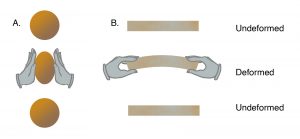 Figure 3-1. Elasticity. (a) An inflated balloon is squeezed between two hands, changing its shape. If the hands are removed, the balloon returns to its earlier shape. (b) A thin board is bent into a curved shape. If the hands bending the board are removed, the board returns to its original shape. The balloon and board are both elastic. |
A video element has been excluded from this version of the text. You can watch it online here: http://pb.libretexts.org/earry/?p=133 |
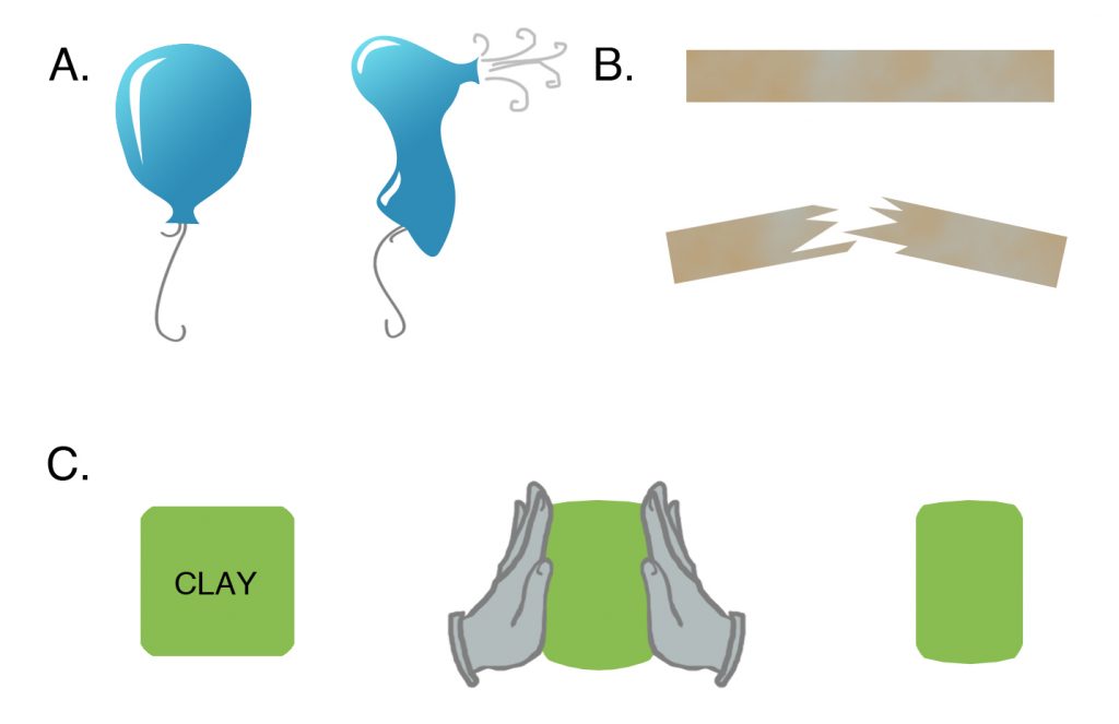 Figure 3-2. (a) When the balloon is squeezed too hard, it pops. (b) When the board is bent too much, it breaks. These are examples of brittle fracture. (c) When a piece of bubble gum or Silly Putty is squeezed between two hands, it deforms. When the hands are removed, it stays in the same deformed shape. This is called ductile deformation. |
If you blow up a balloon, the addition of air causes the balloon to expand. If you then squeeze the balloon with your hands (Figure 3-1, left), the balloon will change its shape. Removing your hands causes the balloon to return to its former shape (Figure 3-1, left). If you take a thin board and bend it with your hands (Figure 3-1, right), the board will deform. If you let the board go, it will straighten out again. These are examples of a property of solids called elasticity. When air is blown into the balloon, or when the balloon is squeezed, or when the board is bent, strain energy is stored up inside the rubber walls of the balloon and within the board. When the balloon is released, or the board is let go, the strain energy is released as balloon and board return to their former shapes.
But if the balloon is blown up even further, it finally reaches a point where it can hold no more air, and it bursts (Figure 3-2, upper left). The strain energy is released in this case, too, but it is released abruptly, with a pop. Instead of returning to its former size, the balloon breaks into tattered fragments. In the same way, if the small board is bent too far, it breaks with a snap as the strain energy is released (Figure 3-2, upper right).
It is not so easy to picture rocks as being elastic, but they are. If a rock is squeezed in a laboratory rock press, it behaves like a rubber ball, changing its shape slightly. When the pressure of the rock press is released, the rock returns to its former shape, just as the balloon or the board does, as shown in Figure 3-1. But if the rock press continues to bear down on the rock with greater force, ultimately the rock will break, like the balloon or the board in Figure 3-2.
This elastic behavior is characteristic of most rocks in the brittle crust, shallower than the brittle-ductile transition, as shown in Figure 2-1. Rocks at greater depths commonly do not break by brittle fracture but deform like bubble gum or like the geologist’s favorite toy, Silly Putty. When a piece of Silly Putty is squeezed together, it deforms permanently; it does not return to its original shape after the squeezing hands are removed (Figure 3-2, bottom).
A video element has been excluded from this version of the text. You can watch it online here: http://pb.libretexts.org/earry/?p=133
A video element has been excluded from this version of the text. You can watch it online here: http://pb.libretexts.org/earry/?p=133
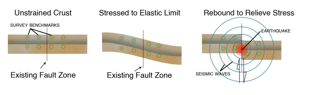
After the great San Francisco Earthquake of 1906 on the San Andreas Fault, Professor Harry F. Reid of Johns Hopkins University, a member of Andrew Lawson’s State Earthquake Investigation Commission, compared two nineteenth-century land surveys on both sides of the fault (Figure 3-3, left and center) with a new survey taken just after the earthquake (Figure 3-3, right). These survey comparisons showed that widely separated survey benchmarks on opposite sides of the fault had moved more than 10 feet (3.2 meters) with respect to each other even before the earthquake, and this slow movement was in the same direction as the sudden movement during the earthquake. Based on these observations, Reid proposed his elastic rebound theory, which states that the Earth’s crust acts like the bent board mentioned earlier. Strain accumulates in the crust until it causes the crust to rupture in an earthquake, like the breaking of the board and the bursting of the balloon.
Another half-century would pass before we would understand why the strain had built up in the brittle crust before the San Francisco Earthquake. We know now that it is due to plate tectonics. The Pacific Plate is slowly grinding past the North America Plate along the San Andreas Fault. But the San Andreas Fault, where the two plates are in contact, is stuck, and so the crust deforms elastically, like bending the board. The break is along the San Andreas Fault because it is relatively weak compared to other parts of the two plates that have not been broken repeatedly. A section of the fault that is slightly weaker than other sections gives way first, releasing the plate-tectonic strain as an earthquake.
If we knew the crustal strengths of various faults, and if we also knew the exact rate at which strain is building up in the crust at these faults, we could then forecast when the next earthquake would strike, an idea that occurred to Harry Reid. We are beginning to understand the rate at which strain builds up on a few of our most hazardous faults, like the San Andreas Fault. But we have very little confidence in our knowledge of the crustal strength that must be overcome to produce an earthquake. The crust is stronger in some places along the fault than others, and crustal strengths are probably different on the same part of a fault at different times in its history. This makes it difficult to forecast when the next earthquake will strike the San Andreas Fault, even though we know more about its earthquake history than any other fault on Earth.

3. A Classification of Faults
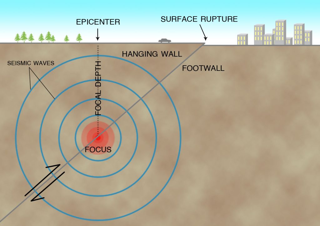
Most damaging earthquakes form on faults at a depth of five miles or more in the Earth’s crust, too deep to be observed directly. But most of these faults are also exposed at the surface where they may be studied by geologists. Larger earthquakes may be accompanied by surface movement on these faults, damaging or destroying human-made structures under which they pass.
Some faults are vertical, so that an earthquake at 10 miles depth is directly beneath the fault at the surface where rupture of the ground can be observed. Other faults dip at a low angle, so that the fault at the surface may be several miles away from the point on the Earth’s surface directly above the earthquake (Figure 3-4). Where the fault has a low dip or inclination, the rock above the fault is called the hanging wall, and the rock below the fault is called the footwall. These are terms that were first coined by miners and prospectors. Valuable ore deposits are commonly found in fault zones, and miners working underground along a fault zone find themselves standing on the footwall, with the hanging wall over their heads.
If the hanging wall moves up or down during an earthquake, the fault is called a dip-slip fault (Figure 3-4). If the hanging wall moves sideways, parallel with the Earth’s surface, as shown in Figure 3-3, 3-5, and 3-6, the fault is called a strike-slip fault.
There are two kinds of strike-slip fault, right-lateral and left-lateral. If you stand on one side of a right-lateral fault, objects on the other side of the fault appear to move to your right during an earthquake (Figure 3-5a, b). The San Andreas Fault is the world’s best-known example of a right-lateral fault (Figure 3-5a). At a left-lateral fault, objects on the other side of the fault appear to move to your left (Figure 3-6). Some of the faults off the coast of Oregon and Washington are left-lateral faults (Figure 4-1, following chapter).
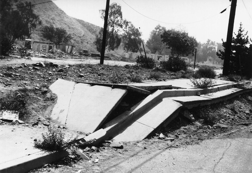
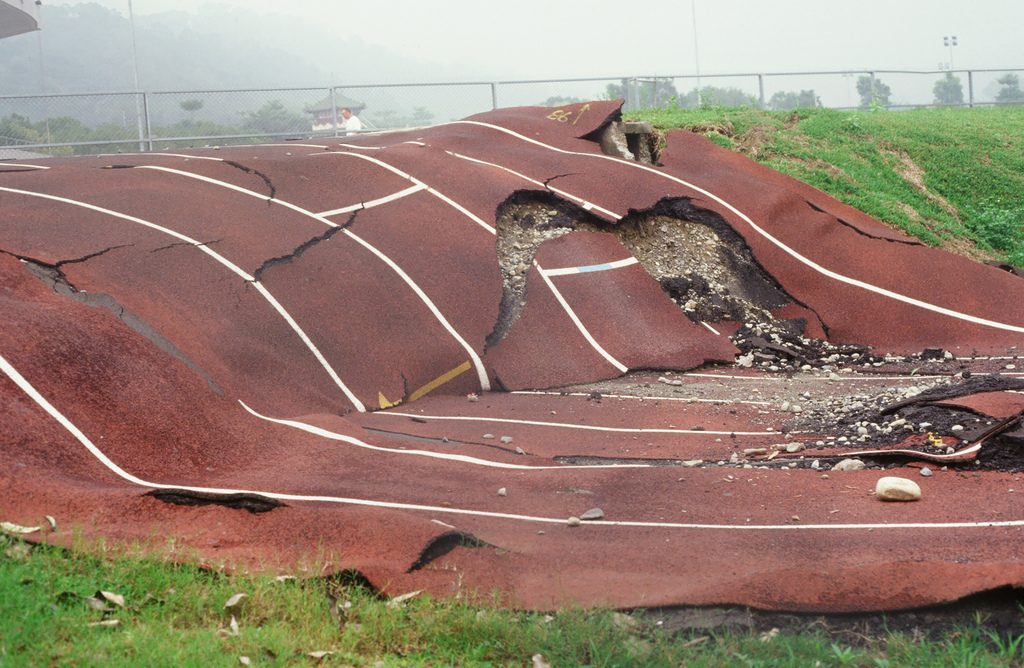
If the hanging wall of a dip-slip fault moves down with respect to the footwall, it is called a normal fault (Figure 3-7). This happens when the crust is being pulled apart, as in the case of faults bordering Steens Mountain in southeastern Oregon, or at sea-floor spreading centers. If the hanging wall moves up with respect to the footwall, it is called a reverse fault (Figure 3-8). This happens when the crust is jammed together. The Cascadia Subduction Zone, where the Juan de Fuca and Gorda oceanic plates are driving beneath the continent, is a very large-scale example of a reverse fault. The 1971 Sylmar Earthquake ruptured the San Fernando Reverse Fault, buckling sidewalks and raising the ground, as shown in Figure 3-8a. The 1999 Chi-Chi, Taiwan, Earthquake was accompanied by surface rupture on a reverse fault, including the rupture across a running track at a high school (Figure 3-8b). The Seattle Fault, extending east-west through downtown Seattle, is a reverse fault. Where the dip of a reverse fault is very low, it is called a thrust fault.
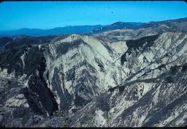
The 1983 Coalinga Earthquake in the central Coast Ranges and the 1994 Northridge Earthquake in the San Fernando Valley, both in California, were caused by rupture on reverse faults, but these faults did not reach the surface. Reverse faults that do not reach the surface are called blind faults, and if they have low dips, they are called blind thrusts. In many cases, such faults are expressed at the Earth’s surface as folds in rock. An upward fold in rock is called an anticline(Figure 3-9), and a downward fold is called asyncline. Before these two earthquakes, geologists thought that anticlines and synclines form slowly and gradually and are not related to earthquakes. Now it is known that they may hide blind faults that are the sources of earthquakes. Such folds cover blind faults in the linear ridges in the Yakima Valley of eastern Washington.
Figure 3-10a is a summary diagram showing the four types of faults that produce earthquakes: left-lateral strike-slip fault, right-lateral strike-slip fault, normal fault, and reverse fault. Figure 2-10b shows a blind reverse fault, the special type of reverse fault that does not reach the surface but is manifested at the surface as an anticline or a warp.
A video element has been excluded from this version of the text. You can watch it online here: http://pb.libretexts.org/earry/?p=133 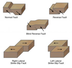 Figure 3-10a. A classification of faults. Top, dip-slip faults. Left, normal fault. Right, reverse fault. Middle, left-lateral and right-lateral strike-slip faults. Bottom, oblique-slip fault, with a component of dip slip and strike slip. |  Figure 3-10b. Blind reverse fault. Fault does not reach the surface; instead, displacement on fault is expressed as a fold. Winnowing action of bottom currents over a seafloor topographic (bathymetric) high. |
4. Paleoseismology: Slip Rates and Earthquake Recurrence Intervals
Major earthquakes are generally followed by aftershocks, some large enough to cause damage and loss of life on their own. The aftershocks are part of the earthquake that just struck, like echoes, but last for months and even years. But if you have just suffered through an earthquake, the aftershocks may cause you to ask: when will the next earthquake strike? I now restate this question: when will the next large earthquake (as opposed to an aftershock) strike the same section of fault?
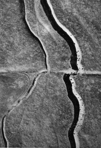
The San Fernando Valley in southern California had an earthquake in 1994, twenty-three years after it last experienced one in 1971. But these earthquakes were on different faults: the 1971 earthquake had surface rupture, the 1994 earthquakes did not. That is not the question I ask here. To answer my question, the geologist tries to determine the slip rate, the rate at which one side of a fault moves past the other side over many thousands of years and many earthquakes. This is done by identifying and then determining the age of a feature like a river channel that was once continuous across the fault but is now offset by it, like the examples in Figure 3-5a.
It is also necessary for us to identify and determine the ages of earthquakes that struck prior to our recorded history, a science called paleoseismology. For example, in central California, Wallace Creek is offset 420 feet (130 meters) across the San Andreas Fault. Sediments deposited in the channel of Wallace Creek prior to its offset are 3,700 years old, based on radiocarbon dating of charcoal in the deposits. The slip rate is the amount of the offset, 420 feet, divided by the age of the channel that is offset, 3,700 years, a little less than 1.4 inches (35 millimeters) per year.
Wallace Creek crosses that part of the San Andreas Fault where strike-slip offset during the great Fort Tejon Earthquake of 1857 was 30-40 feet. How long would it take for the fault to build up as much strain as it released in 1857? To find out, divide the 1857 slip, 30-40 feet, by the slip rate, 1.4 inches per year, to get 260 to 340 years, which is an estimate of the average earthquake recurrence interval for this part of the fault. (I round off the numbers because the age of the offset Wallace Creek, based on radiocarbon dating, and the amount of its offset are not precisely known.) Paleoseismologic investigation of backhoe trench excavations shows that the last earthquake to strike this part of the fault prior to 1857 was around the year 1480, an interval of 370 to 380 years, which agrees with our calculations within our uncertainty of measurement. This is reassuring because the lowest estimate of the recurrence interval, 260 years, won’t end until after the year 2100.
Crustal faults in the Pacific Northwest have much slower slip rates, and so the earthquake recurrence times are much longer. Say that we learned that a reverse fault has a slip rate of 1/25 inch (1 millimeter) per year, and we conclude from a backhoe trench excavation across the fault that an earthquake on the fault will cause it to move 10 feet (120 inches). The return time would be three thousand years. Could we use that information to forecast when the next earthquake would occur on that fault?
Unfortunately, this question is not easy to answer because the faults and the earthquakes they produce are not very orderly. For example, the 1812 and 1857 earthquakes on the same section of the San Andreas Fault ruptured different lengths of the fault, and their offsets were different. Displacements on the same fault during the same earthquake differ from one end of the rupture to the other. The recurrence intervals differ as well. We were reassured by the recurrence interval of 370 to 380 years between the 1857 earthquake and a prehistoric event around A.D. 1480, but the earthquake prior to A.D. 1480 struck around A.D. 1350, a recurrence interval of only 130 years. For a fault with an average recurrence interval of three thousand years, the irregularity in return times could be more than a thousand years, so that the average recurrence interval would have little value in forecasting the time of the next earthquake on that section of fault.
We can give a statistical likelihood of an earthquake striking a given part of the San Andreas Fault in a certain time interval after the last earthquake (see Chapter 7), but we can’t nail this down any closer because of the poorly understood variability in strength of fault zones, variability in time as well as position on the fault. Another difficulty is in our use of radiocarbon dating to establish the timing of earlier earthquakes. Charcoal may be rare in the faulted sediments we are studying. And radiocarbon doesn’t actually date an earthquake. It dates the youngest sediments cut by a fault and the oldest unfaulted sediments overlying the fault, assuming that these sediments have charcoal suitable for dating.
5. What Happens During an Earthquake?
Crustal earthquakes start at depths of five to twelve miles, typically in that layer of the Earth’s crust that is strongest due to burial pressure, just above the brittle-ductile transition, the depth below which temperature weakening starts to take effect (Figure 2-1). Slab earthquakes like the Nisqually Earthquake of 2001 start in the Juan de Fuca Plate underlying the continent, at greater depths but still in brittle rock. These depths are too great for us to study the source areas of earthquakes directly by deep drilling, and so we have to base our understanding on indirect evidence. We do this by studying the detailed properties of seismic waves that pass through these crustal layers, or by subjecting rocks to laboratory tests at temperatures and pressures expected at those depths. And some ancient fault zones have been uplifted and eroded in the millions of years since faulting took place, allowing us to observe them directly at the surface and make inferences on how ancient earthquakes may have occurred on them.
A video element has been excluded from this version of the text. You can watch it online here: http://pb.libretexts.org/earry/?p=133 |
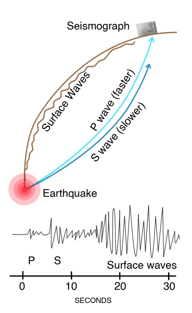 Figure 3-11. An earthquake produces P waves, or compressional waves, that travel faster and reach the seismograph first, and S waves, or shear waves, that are slower. Both are transmitted within the Earth and are called body waves. Even slower are surface waves that run along the surface of the earth and do a lot of the damage. The earthquake focus is the point within the Earth where the earthquake originates. The epicenter is a point on the surface directly above the focus. The diagram below is a seismogram, reading from left to right, showing that the P wave arrives first, followed by the S wave and then by surface waves. |
An earthquake is most likely to rupture the crust where it previously has been broken at a fault, because a fault zone tends to be weaker than unfaulted rock around it. The Earth’s crust is like a chain, only as strong as its weakest link. Strain has been building up elastically, and now the strength of the faulted crust directly above the zone where temperature weakening occurs is reached. Suddenly, this strong layer fails, and the rupture races sideways and upward toward the surface, breaking the weaker layers above it, and even downward into crust that would normally behave in a ductile manner. The motion in the brittle crust produces friction, which generates heat that may be sufficient to melt the rock in places. In cases where the rupture only extends for a mile or so, the earthquake is a relatively minor one, like the 1993 Scotts Mills Earthquake east of Salem, Oregon. But in rare instances, the rupture keeps going for hundreds of miles, and a great earthquake like the 1906 San Francisco Earthquake or the 2002 Denali, Alaska, Earthquake is the result. At present, scientists can’t say why one earthquake stops after only a small segment of a fault ruptures, but another segment of fault ruptures for hundreds of miles, generating a giant earthquake.
The rupture causes the sudden loss of strain energy that the rock had built up over hundreds of years, equivalent to the snap of the board or the pop of the balloon. The shock radiates out from the rupture as seismic waves, which travel to the surface and produce the shaking we experience in an earthquake (Figure 3-11). These waves are of three basic types: P waves (primary waves), S waves (secondary or shear waves), and surface waves. P and S waves are called body waves because they pass directly through the Earth, whereas surface waves travel along the Earth’s surface, like the ripples in a pond when a stone is thrown into it.
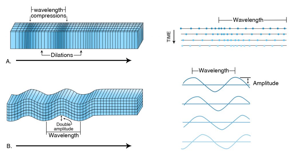
P and S waves are fundamentally different (Figure 3-12). A P wave is easily understood by a pool player, who “breaks” a set of pool balls arranged in a tight triangle, all touching. When the cue ball hits the other balls, the energy of striking momentarily compresses the next ball elastically. The compression is transferred to the next ball, then to the next, until the entire set of pool balls scatters around the table. The elastic deformation is parallel to the direction the wave is traveling, as shown by the top diagram in Figure 3-12. P waves pass through a solid, like rock, and they can also pass through water or air. When earthquake waves pass through air, sometimes they produce a noise.
An S wave can be imagined by tying one end of a rope to a tree. Hold the rope tight and shake it rapidly from side to side. You can see what looks like waves running down the rope toward the tree, distorting the shape of the rope. In the same fashion, when S waves pass through rock, they distort its shape. The elastic deformation is at right angles to the direction the wave travels, as shown by the bottom diagram in Figure 3-12. S waves cannot pass through liquid or air, and they would not be felt aboard a ship at sea.
A video element has been excluded from this version of the text. You can watch it online here: http://pb.libretexts.org/earry/?p=133 |
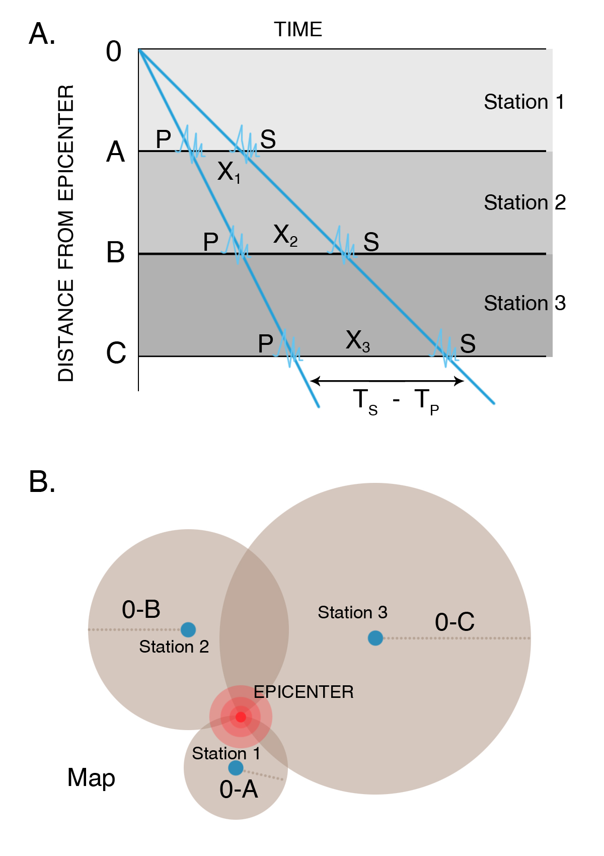 Figure 3-12. Two views of (a) P waves and (b) S waves, all moving from left to right. A P wave moves by alternately compressing and dilating the material through which it passes, somewhat analogous to stop-and-go traffic on the freeway during rush hour. An S wave moves by shearing the material from side to side, analogous to flipping a rope tied to a tree. Note the illustration of wavelength for P and S waves and amplitude for S waves. The number of complete wavelengths to pass a point in a second is the frequency. |
Because S waves are produced by sideways motion, they are slower than P waves, and the seismologist uses this fact to tell how far it is from the seismograph to the earthquake (Figure 3-13). The seismogram records the P wave first, then the S wave. If the seismologist knows the speed of each wave, then by knowing that both waves started at the same time, it is possible to work out how far the earthquake waves have traveled to reach the seismograph. If we can determine the distance of the same earthquake from several different seismograph stations, we are able to locate the epicenter, which is the point on the Earth’s surface directly above the earthquake focus. The focus or hypocenter is the point beneath the Earth’s surface where the crust or mantle first ruptures to cause an earthquake (Figure 3-4). The depth of the earthquake below the surface is called its focal depth.
A modern three-component seismograph station provides more information about an earthquake source than a single-component seismograph because it consists of three separate seismometers, one measuring motion in an east-west direction, one measuring north-south motion, and one measuring up-down motion. An east-west seismometer, for example, can tell if the wave is coming from an easterly or westerly direction, and a seismograph in Seattle could distinguish an earthquake on the Cascadia Subduction Zone to the west from an earthquake in the Pasco Basin east of the Cascades.
The surface waves are more complex. After reaching the surface, much earthquake energy will run along the surface, causing the ground to go up and down, or sway from side to side. Some people caught in an earthquake have reported that they could actually see the ground moving up and down, like an ocean wave, but faster.
An earthquake releases a complex array of waves, with great variation in frequency, which is the number of waves to pass a point in a second. A guitar string vibrates many times per second, but it takes successive ocean waves many seconds to reach a waiting surfer. The ocean wave has a low frequency, and the guitar string vibrates at a high frequency. An earthquake can be compared to a symphony orchestra, with cellos, bassoons, and bass drums producing sound waves that vibrate at low frequencies, and piccolos, flutes, and violins that vibrate at high frequencies. It is only by use of high-speed computers that a seismologist can separate out the complex vibrations produced by an earthquake and begin to read and understand the music of the spheres.
A video element has been excluded from this version of the text. You can watch it online here: http://pb.libretexts.org/earry/?p=133
To explain this, I return to my piece of Silly Putty (Figure 3-2). Silly Putty can be stretched out like bubble gum when it is pulled slowly. Hang a piece of Silly Putty over the side of a table, and it will slowly drip to the floor under its own weight, like soft tar (ductile flow). Yet it has another, seemingly contradictory, property when it is deformed rapidly. It will bounce like a ball, indicating that it can be elastic. If Silly Putty is stretched out suddenly, it will break, sometimes into several pieces (brittle fracture).
The difference is whether the strain is applied suddenly or slowly. When strain is applied quickly, Silly Putty will absorb strain elastically (it will bounce), or it will shatter, depending on whether the strain takes it past its breaking point. Earthquake waves deform rock very quickly, and like Silly Putty, the rock behaves like an elastic solid. If strain is applied slowly, Silly Putty flows, almost like tar. This is the way the asthenosphere and lower crust work. The internal currents that drive the motion of plate tectonics are extremely slow, inches per year or less, and at those slow rates, rock flows.
Furthermore, when a fault ruptures the brittle crust just above the brittle-ductile transition, the fault rupture may propagate downward into crust that behaves in a brittle fashion because the fault rupture is generated at high speed, in contrast to its response to the slow deformation of plate tectonics. We will return to this subject in Chapter 4, where we consider the behavior of the Cascadia Subduction Zone, in which the plate boundary consists of material closer to the surface that is elastic or subject to brittle fracture under all conditions, a deeper layer that is ductile under all conditions, and an intermediate, or transitional, layer that is ductile when stress is applied slowly, at the rates of plate tectonics, but is brittle when stress is applied rapidly as an earthquake-generating fault propagates downward. But even the deepest layer is elastic to the propagation of seismic body waves.
6. Measuring an Earthquake
a. Magnitude
The chorus of high-frequency and low-frequency seismic waves that radiate out from an earthquake indicates that no single number can characterize an earthquake, just as no single number can be used to describe a Yakima Valley wine or a sunset view of Mt. Rainier or Mt. Hood.
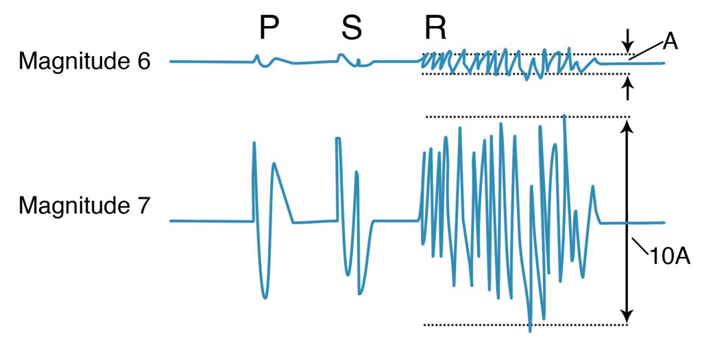
The size of an earthquake was once measured largely on the basis of how much damage was done. This was unsatisfactory to Caltech seismologist Charles Richter, who wanted a more quantitative measure of earthquake size, at least for southern California. Following up on earlier work done by the Japanese, Richter in 1935 established a magnitude scale based on how much a seismograph needle is deflected by a seismic wave generated by an earthquake about sixty miles (a hundred kilometers) away (Figure 3-14). Richter used a seismograph specially designed by seismologist Harry Wood and astronomer John Anderson to record local earthquakes in southern California. This seismograph was best suited for those waves that vibrated with a frequency of about five times per second, which is a bit like measuring how loud an orchestra is by how loud it plays middle C. Nonetheless, it enabled Richter and his colleagues to distinguish large, medium-sized, and small earthquakes in California, which was all they wanted to do. Anderson was an astronomer, and the seismograph was built at the Mt. Wilson Observatory, which may account for the word magnitude, a word that also expresses how bright a star is.
Complicating the problem for the lay person is that Richter’s scale is logarithmic, which means that an earthquake of magnitude 5 would deflect the needle of the Wood-Anderson seismograph ten times more than an earthquake of magnitude 4 (Figure 3-14). And an increase of one magnitude unit represents about a thirty-fold increase in release of stored-up seismic strain energy. So the Olympia, Washington, Earthquake of 7.1 on April 13, 1949, would be considered to have released the energy of more than thirty earthquakes the size of the Klamath Falls, Oregon, Earthquake of September 20, 1993, which was magnitude 6.
A video element has been excluded from this version of the text. You can watch it online here: http://pb.libretexts.org/earry/?p=133
Richter never claimed that his magnitude scale, now called local magnitude and labeled ML, was an accurate measure of earthquakes. Nonetheless, the Richter magnitude scale caught on with the media and the general public, and it is still the first thing that a reporter asks a professional about an earthquake: “How big was it on the Richter scale?” The Richter magnitude scale works reasonably well for small to moderate-size earthquakes, but it works poorly for very large earthquakes, the ones we call great earthquakes. For these, other magnitude scales are necessary.
To record earthquakes at seismographs thousands of miles away, seismologists had to use long-period (low-frequency) waves, because the high-frequency waves recorded by Richter on the Wood-Anderson seismographs die out a few hundred miles away from the epicenter. To understand this problem, think about how heavy metal music is heard a long distance away from its source, a live band or a boom box. Sometimes when my window is open on a summer evening, I can hear a faraway boom box in a passing car, but all I can hear are the very deep, or low-frequency, tones of the bass guitar, which transmit through the air more efficiently than the treble (high-frequency) guitar notes or the voices of the singers. In this same way, low-frequency earthquake waves can be recorded thousands of miles away from the earthquake source, so that we were able to record the magnitude 9 Tohoku-oki earthquake in Japan on our seismograph in Corvallis, Oregon. Low-frequency body waves pass through the Earth and are used to study its internal structure, analogous to X-rays of the human body. A body-wave magnitude is called mb.
A commonly used earthquake scale is the surface wave magnitude scale, or MS, which measures the largest deflection of the needle on the seismograph for a surface wave that takes about twenty seconds to pass a point (which is about the same frequency as some ocean waves).
The magnitude scale most useful to professionals is the moment magnitude scale, or MW, which comes closest to measuring the true size of an earthquake, particularly a large one. This scale relates magnitude to the area of the fault that ruptures and the amount of slip that takes place on the fault. For many very large earthquakes, this can be done by measuring the length of the fault that ruptures at the surface and figuring out how deep the zone of aftershocks extends, thereby calculating the area of the rupture. The amount of slip can be measured at the surface as well. The seismologist can also measure MW by studying the characteristics of low-frequency seismic waves, and the surveyor or geodesist (see section 7 of this chapter) can measure it by remeasuring the relative displacement of survey benchmarks immediately after an earthquake to work out the distortion of the ground surface and envisioning a subsurface fault that would produce the observed distortion (see below).
For small- to intermediate-size earthquakes, the magnitude scales are designed so that there is relatively little difference between Richter magnitude, surface-wave magnitude, and moment magnitude. But for very large earthquakes, the difference is dramatic. For example, both the 1906 San Francisco Earthquake and the 1964 Alaska Earthquake had a surface-wave magnitude of 8.3. However, the San Francisco Earthquake had a moment magnitude of only 7.9, whereas the Alaska Earthquake had a moment magnitude of 9.2, which made it the second-largest earthquake of the twentieth century. The surface area of the fault rupture in the Alaska Earthquake was the size of the state of Iowa!
b. Intensity
Measuring the size of an earthquake by the energy it releases is all well and good, but it is still important to measure how much damage it does at critical places (such as where you or I or our loved ones happen to be when the earthquake strikes). This measurement is called earthquake intensity, which is measured by a Roman numeral scale (Table 3-1). Intensity III means no damage, and not everybody feels it. Intensity VII or VIII involves moderate damage, particularly to poorly constructed buildings, while Intensity IX or X causes considerable damage. Intensity XI or XII, which fortunately is rare, is characterized by nearly total destruction.
Earthquake intensities are based on a post-earthquake survey of a large area. Damage is noted, and people are questioned about what they felt. An intensity map is a series of concentric lines, irregular rather than circular, in which the highest intensities are generally (but not always) closest to the epicenter of the earthquake. For illustration, an intensity map is shown for the 1993 Scotts Mills Earthquake in the Willamette Valley of Oregon (Figure 3-15). High intensities were recorded near the epicenter, as expected. But intensity can also be influenced by the characteristics of the ground. Buildings on solid rock tend to fare better (and thus are subjected to lower intensities) than buildings on thick soft soil. The Intensity VI contour bulges out around the capital city of Salem, and the Intensity V contour bends south to include the city of Albany. Both are along the Willamette River (dotted line in Figure 3-15), where soft river deposits increased strong shaking. The effect of soft soils is discussed further in Chapter 8.
| Modified Mercalli Intensity Scale |
|---|
| I Not felt except by a very few, under especially favorable circumstances. |
| II Felt only by a few persons at rest, especially on upper floors of buildings. Delicately suspended objects may swing. |
| III Felt quite noticeably indoors, especially on upper floors of buildings, but many people do not recognize it as an earthquake. Standing automobiles may rock slightly. Vibrations like the passing of a truck. |
| IV During the day, felt indoors by many, outdoors by few. At night, some awakened. Dishes, windows, doors disturbed; walls make creaking sound. Sensation like heavy truck striking building. Standing automobiles rocked noticeably. |
| V Felt by nearly everyone; many awakened. Some dishes, windows, etc. broken; cracked plaster in a few places; unstable objects overturned. Disturbance of trees, poles, and other tall objects sometimes noticed. Pendulum clocks may stop. |
| VI Felt by all, many frightened and run outdoors. Some heavy furniture moved; a few instances of fallen plaster and damaged chimneys. Damage slight; masonry D cracked. |
| VII Everybody runs outdoors. Damage negligible in buildings of good design and construction; slight to moderate in well-built ordinary structures; considerable in poorly built or badly designed structures (masonry D); some chimneys broken. Noticed by persons driving cars. |
| VIII Damage slight in specially designed structure; no damage to masonry A, some damage to masonry B, considerable damage to masonry C with partial collapse. panel walls thrown out of frame structures. Fall of chimneys, factory stacks, columns, monuments, walls. Frame houses moved off foundations if not bolted. Heavy furniture overturned. Sand and mud ejected in small amounts. Changes in well water. Persons driving cars disturbed. |
| IX Damage considerable in specially designed structures; well-designed frame structures thrown out of plumb; great in substantial buildings, with partial collapse. Masonry B seriously damaged, masonry C heavily damaged, some with partial collapse, Masonry D destroyed. Buildings shifted off foundations. Ground cracked conspicuously. Underground pipes broken. |
| X Some well-built wooden structures destroyed; most masonry and frame structures destroyed with foundations; ground badly cracked. Rails bent. Landslides considerable from river banks and steep slopes. Shifted sand and mud. Water splashed over banks. |
| XI Few, if any, masonry structures remain standing. Bridges destroyed. Broad fissures in ground. Underground pipelines completely our of service. Earth slumps and land slips in soft ground. Rails bent greatly. |
| XII Damage total. Waves seen on ground surface. Lines of sight and level distorted. Objects thrown into the air. |
| Masonry A Good workmanship, mortar, and design; reinforced, especially laterally, and bout together using steel, concrete, etc. Masonry B Good workmanship and mortar, reinforce, but not designed in detail to resist lateral forces. Masonry C Ordinary workmanship and mortar, no extreme weakness like failing to tie in at corners, but neither reinforced nor designed against horizontal forces. Masonry D |
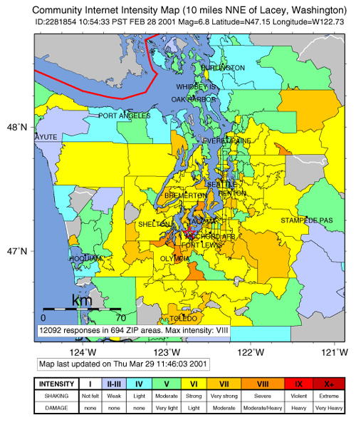
In the Pacific Northwest, creating an intensity map by the use of questionnaires is now done on the Internet. You can contribute to science. If you feel an earthquake, go to http://www.ess.washington.edu and click on Pacific Northwest Earthquakes, which will take you to the Pacific Northwest Seismograph Network. Click on Report an Earthquake. This brings up the phrase, Did You Feel It? Click on your state and you can fill out a report and submit it electronically. The resulting map shows intensity in color, by zip code, and is called the Community Internet Intensity Map (CIIM). Figure 3-16 shows the CIIM for the 2001 Nisqually Earthquake. An earthquake of M 3.7 near Bremerton, Washington, on May 29, 2003, drew more than one thousand responses in the first twenty-four hours.
Figure 3-17 relates earthquake intensity to the maximum amount of ground acceleration (peak ground acceleration, or PGA) that is measured with a special instrument called a strong-motion accelerograph. Acceleration is measured as a percentage of the Earth’s gravity. A vertical acceleration of one g would be just enough to lift you (or anything else) off the ground. Obviously, this would have a major impact on damage done by an earthquake at a given site. Peak ground velocity (PGV) is also routinely measured.
In the Pacific Northwest, creating an intensity map by use of questionnaires is now done on the Internet. If you feel an earthquake, go to http://www.ess.washington.edu and click on Pacific Northwest Earthquakes, which will take you to the Pacific Northwest Seismograph Network. Click on Report an Earthquake. This brings up the phrase, Did You Feel It? Click on your state and you can fill out a report and submit it electronically. The map that results shows intensity by zip code and is called the Community Internet Intensity Map (CIIM). Figure 3-16 shows the CIIM for the 2001 Nisqually Earthquake. An earthquake of M 3.7 near Bremerton, Washington, on May 29, 2003, drew more than one thousand responses in the first twenty-four hours.
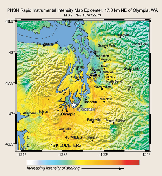
The Internet-derived intensity map is not generated fast enough to be of use to emergency managers, who need to locate quickly the areas of highest intensity, and thus the areas where damage is likely to be greatest. What resources must be mobilized, and where should they be sent? The TriNet Project was developed for southern California by the U.S. Geological Survey (USGS), Caltech, and the California Geological Survey with support from the Federal Emergency Management Agency (FEMA), taking advantage of the large number of strong-motion seismographs in the state, a detailed knowledge of active faults of the region, and of soil types likely to result in high accelerations. After the Northridge Earthquake of 1994, this project developed ShakeMap, which takes the calculated magnitude, depth, causative fault, direction of rupture propagation, and soil types to produce an intensity map within five minutes of the earthquake. The ShakeMap software was installed at the Pacific Northwest Seismograph Network at the University of Washington in January 2001, one month before the Nisqually Earthquake, and was still in test mode when that earthquake struck. The ShakeMap for this earthquake, which was made available to the public one day after the earthquake, is shown as Figure 3-17. You can access a ShakeMap, even for smaller earthquakes, through http://www.trinet.org/shake or through the Pacific Northwest Seismograph Network website.
As pointed out above, Intensities VII and VIII may result in major damage to poorly constructed buildings whereas well-constructed buildings should ride out those intensities with much less damage. This points out the importance of earthquake-resistant construction and strong building codes, discussed further in Chapters 11 and 12. Except for adobe, nearly all buildings will ride out intensities of VI or less, even if they are poorly constructed. For the rare occasions when intensities reach XI or XII, many buildings will fail, even if they are well constructed. But for the more common intensities of VII through X, earthquake-resistant construction will probably mean the difference between collapse of the building, with loss of life, and survival of the building and its inhabitants.
Measurements of intensity are the only way to estimate the magnitudes of historical earthquakes that struck before the development of seismographs. Magnitude estimates based on intensity data have been made for decades, but these were so subjective that magnitude estimates and epicenter locations made in this way were unreliable. For example, the epicenter of the poorly understood earthquake of December 14, 1872 has been placed at many locations in northeastern Washington and even in southern British Columbia, with magnitude estimates as high as M 7.4. Can these estimates be made more quantitative, and thereby more useful in earthquake hazard estimates?
Bill Bakun and Carl Wentworth of the USGS figured out a way to do it. First, they had to cope with the behavior of seismic waves passing through parts of the Earth that react to seismic waves in different ways. Seismic waves die out (attenuate) more rapidly in some parts of the Earth than in others. It’s like hitting a sawed log with a hammer and listening for the sound at the other end. If the wood is good, the hammer makes a clean sound. If the wood is rotten, however, the hammer goes “thunk”. By measuring the attenuation (“thunkiness”) and wave speeds of more recent earthquakes that have had magnitudes determined by seismographs, Bakun and Wentworth were able to calibrate the behavior of the Earth’s crust in the vicinity of pre-instrumental earthquakes in the same region. The magnitude measured in this way is called intensity magnitude, or MI.
Bakun teamed with several colleagues, including Ruth Ludwin of the University of Washington and Margaret Hopper of the USGS, who had already done a study of the 1872 earthquake, and analyzed twentieth-century earthquakes with instrumentally determined magnitudes both east and west of the Cascades to take into account the different behavior of the Earth’s crust in western as compared to eastern Washington. They compared the intensities from these modern earthquakes with the intensities reported from the 1872 earthquake at seventy-eight locations to find the epicenter and magnitude that best matched the pattern of intensity observed in 1872. The earthquake, they determined, was located south of Lake Chelan with MI estimated as 6.8. (This earthquake is discussed further in Chapter 6.)
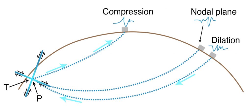
c. Fault-Plane Solutions
In the early days of seismography, it was enough to locate an earthquake accurately and to determine its magnitude. But seismic waves contain much more information, including the determination of the type of faulting. The seismogram shows that the first motion of an earthquake P-wave is either a push toward the seismograph or a pull away from it. With the modern three-component networks in the Northwest and adjacent parts of Canada, it is possible to determine the push or pull relationship at many stations, leading to information about whether the earthquake is on a reverse fault, a normal fault, or a strike-slip fault (as illustrated in Figure 3-18, which indicates the earthquakes was on a normal fault in which the earthquakes wave pushed outward horizontally from the hypocenter, similar to the 1993 Klamath Falls Earthquake). Most earthquakes are not accompanied by surface faulting, so the fault-plane solutions are the best evidence of the type of fault causing the earthquake. The fault generating the September 1993 Klamath Falls, Oregon, Earthquakes did not rupture the surface, but their fault-plane solutions showed that they were caused by rupture of a normal fault striking approximately north-northwest, in agreement with the local geology (for further discussion, see Chapter 6). Seismic waves recorded digitally on broadband seismographs are able to record many frequencies of seismic waves. These can be analyzed to show that an earthquake may consist of several ruptures within a few seconds of each other, some with very different fault-plane solutions.
A video element has been excluded from this version of the text. You can watch it online here: http://pb.libretexts.org/earry/?p=133
7. Measuring Crustal Deformation Directly:
Tectonic Geodesy
As stated at the beginning of this chapter, Harry F. Reid based his elastic rebound theory on the displacement of survey benchmarks relative to one another. These benchmarks recorded the slow elastic deformation of the Earth’s crust prior to the 1906 San Francisco Earthquake. After the earthquake, the benchmarks snapped back, thereby giving an estimate of tectonic deformation near the San Andreas Fault independent of seismographs or of geological observations. Continued measurements of the benchmarks record the accumulation of strain toward the next earthquake. If geology records past earthquakes and seismographs record earthquakes as they happen, measuring the accumulation of tectonic strain says something about the earthquakes of the future.
Reid’s work means that a major contribution to the understanding of earthquakes can be made by a branch of civil engineering called surveying: land measurements of the distance between survey markers (trilateration), the horizontal angles between three markers (triangulation), and the difference in elevation between two survey markers (leveling).
Surveyors need to know about the effects of earthquakes on property boundaries. Surveying normally implies that the land stays where it is. But if an earthquake is accompanied by a ten-foot strike-slip offset on a fault crossing your property, would your property lines be offset, too? In Japan, where individual rice paddies and tea gardens have property boundaries that are hundreds of years old, property boundaries are offset. A land survey map of part of the island of Shikoku shows rice paddy property boundaries offset by a large earthquake fault in A.D. 1596.
The need to have accurate land surveys leads to the science of geodesy, the study of the shape and configuration of the Earth, a discipline that is part of civil engineering. Tectonic geodesy is the comparison of surveys done at different times to reveal deformation of the crust between the times of the surveys.
Following Reid’s discovery, the U.S. Coast and Geodetic Survey (now the National Geodetic Survey) took over the responsibility for tectonic geodesy, which led them into strong-motion seismology. For a time, the Coast and Geodetic Survey was the only federal agency with a mandate to study earthquakes (see Chapter 13).
After the great Alaska Earthquake of 1964, the USGS began to take an interest in tectonic geodesy as a way to study earthquakes. The leader in this effort was a young geophysicist named Jim Savage, who compared surveys before and after the earthquake to measure the crustal changes that accompanied the earthquake. The elevation changes were so large that along the Alaskan coastline, they could be easily seen without surveying instruments: sea level appeared to rise suddenly where the land went down, and it appeared to drop where the land went up. (Of course, sea level didn’t actually rise or fall, the land level changed.)
Up until the time of the earthquake, some scientists believed that the faults at deep-sea trenches were vertical. But Savage, working with geologist George Plafker, was able to use the differences in surveys to show that the great subduction-zone fault that had generated the earthquake dips gently northward, underneath the Alaskan landmass. Savage and Plafker then studied an even larger subduction-zone earthquake that had struck southern Chile in 1960 (Moment Magnitude Mw 9.5, the largest earthquake ever recorded) and showed that the earthquake fault in the Chilean deep-sea trench dipped beneath the South American continent. Seismologists, using newly established high-quality seismographs set up to monitor the testing of nuclear weapons, confirmed this by showing that earthquakes defined a landward-dipping zone that could be traced hundreds of miles beneath the surface. These became known as Wadati-Benioff zones, named for the seismologists who first described them. All these discoveries were building blocks in the emerging new theory of plate tectonics.
In 1980, Savage turned his attention to the Cascadia Subduction Zone off Washington and Oregon. This subduction zone was almost completely lacking in earthquakes and was thought to deform without earthquakes. But Savage, resurveying networks in the Puget Sound area and around Hanford Nuclear Reservation in eastern Washington, found that these areas were accumulating elastic strain, like areas in Alaska and the San Andreas Fault. Then John Adams, a young New Zealand geologist transplanted to the Geological Survey of Canada, remeasured leveling lines across the Coast Range and found that the coastal region was tilting eastward toward the Willamette Valley and Puget Sound, providing further evidence of elastic deformation. These geodetic observations were critical in convincing scientists that the Cascadia Subduction Zone was capable of large earthquakes, like the subduction zones off southern Alaska and Chile (see Chapter 4).
At the same time, the San Andreas fault system was being resurveyed along a spider web of line-length measurements between benchmarks on both sides of the fault. Resurveys were done once a year, more frequently later in the project. The results confirmed the elastic-rebound theory of Reid, and the large number of benchmarks and the more frequent surveying campaigns added precision that had been lacking before. Not only could Savage and his coworkers determine how fast strain is building up on the San Andreas, Hayward, and Calaveras faults, they were even able to determine how deep within the Earth’s crust the faults are locked.
After an earthquake in the San Fernando Valley near Los Angeles in 1971, Savage releveled survey lines that crossed the surface rupture. He was able to use the geodetic data to map the source fault dipping beneath the San Gabriel Mountains, just as he had done for the Alaskan Earthquake fault seven years before. The depiction of the source fault based on tectonic geodesy could be compared with the fault as illuminated by the distribution of aftershocks and by the surface geology of the fault scarp. This would be the wave of the future in the analysis of California earthquakes.
Still, the land survey techniques were too slow, too cumbersome, and too expensive. A major problem was that the baselines were short, because the surveyors had to see from one benchmark to the other to make a measurement.
The solution to the problem came from space.
First, scientists from the National Aeronautical and Space Administration (NASA) discovered mysterious, regularly spaced radio signals from quasars in deep outer space. By analyzing these signals simultaneously from several radio telescopes as the Earth rotated, the distances between the radio telescopes could be determined to great precision, even though they were hundreds of miles apart. And these distances changed over time. Using a technique called Very Long Baseline Interferometry (VLBI), NASA was able to determine the motion of radio telescopes on one side of the San Andreas Fault with respect to telescopes on the other side. These motions confirmed Savage’s observations, even though the radio telescopes being used were hundreds of miles away from the San Andreas Fault.
Length of baseline ceased to be a problem, and the motion of a radio telescope at Vandenberg Air Force Base could be compared to a telescope in the Mojave Desert, in northeastern California, in Hawaii, in Japan, in Texas, or in Massachusetts. Using VLBI, NASA scientists were able to show that the motions of plate tectonics measured over time spans of hundreds of thousands of years are at the same rate as motions measured for only a few years—plate tectonics in real time.
But there were not enough radio telescopes to equal Savage’s dense network of survey stations across the San Andreas Fault. Again, the solution came from space, this time from a group (called a constellation) of NAVSTAR satellites that orbit the Earth at an altitude of about twelve thousand miles. This developed into the Global Positioning System, or GPS.
GPS was developed by the military so that smart bombs could zero in on individual buildings in Baghdad or Belgrade, but low-cost GPS receivers allow hunters to locate themselves in the mountains and fishing boats to be located at sea. You can install one on the dashboard of your car to find where you are in a strange city. GPS is now widely used in routine surveying. In tectonic geodesy, it doesn’t really matter where we are exactly, but only where we are relative to the last time we measured. This allows us to measure small changes of only a fraction of an inch, which is sufficient to measure strain accumulation. Uncertainties about variations in the troposphere high above the Earth mean that GPS does much better at measuring horizontal changes than it does vertical changes; leveling using GPS is less accurate than leveling based on ground surveys.
NASA’s Jet Propulsion Lab at Pasadena, together with scientists at Caltech and MIT, began a series of survey campaigns in southern California in the late 1980s, and they confirmed the earlier ground-based and VLBI measurements. GPS campaigns could be done quickly and inexpensively, and, like VLBI, it was not necessary to see between two adjacent ground survey points. It was only necessary for all stations to lock onto one or more of the orbiting NAVSTAR satellites.
In addition to measuring the long-term accumulation of elastic strain, GPS was able to measure the release of strain in the 1992 Landers Earthquake in the Mojave Desert and the 1994 Northridge Earthquake in the San Fernando Valley. The survey network around the San Fernando Valley was dense enough that GPS could determine the size and orientation of the source fault plane and the amount of displacement during the earthquake. This determination of magnitude was independent of the fault source measurements made using seismography or geology.
In addition to measuring the long-term accumulation of elastic strain, GPS was able to measure the release of strain in the 1992 Landers Earthquake in the Mojave Desert and the 1994 Northridge Earthquake in the San Fernando Valley. The survey network around the San Fernando Valley was dense enough that GPS could determine the size and orientation of the source fault plane and the amount of displacement during the earthquake. This determination of magnitude was independent of the fault source measurements made using seismography or geology.
By the time of the Landers Earthquake, tectonic geodesists recognized that campaign-style GPS, in which teams of geodesists went to the field several times a year to remeasure their ground survey points, was not enough. The measurements needed to be more frequent, and the time of occupation of individual sites needed to be longer, to increase the level of confidence in measured tectonic changes and to look for possible short-term geodetic changes that might precede an earthquake. So permanent GPS receivers were installed at critical localities that were shown to be stable against other types of ground motion unrelated to tectonics, such as ground slumping or freeze-thaw. The permanent network was not dense enough to provide an accurate measure of either the Landers or the Northridge earthquake, but the changes they recorded showed great promise for the future.
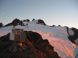
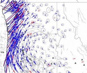
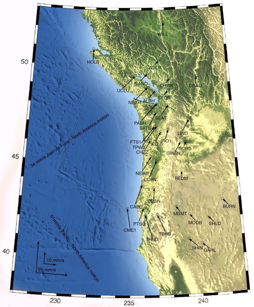
After Northridge, geodetic networks were established in southern California, the San Francisco Bay Area, and the Great Basin area including Nevada and Utah. In the Pacific Northwest, a group of scientists including Herb Dragert of the Pacific Geoscience Centre in Sidney, B.C., and Meghan Miller, then of Central Washington University in Ellensburg, organized networks for the Pacific Northwest called the Pacific Northwest Geodetic Array (PANGA) and Western Canada Deformation Array, building on the ongoing work of Jim Savage and his colleagues at the USGS. Figure 3-19 shows a GPS receiver being used to measure coseismic deformation within the PANGA network, in this case in Olympic National Park, where on eif the early GPS studies in the Northwest was done under the direction of Jim Savage. The permanent arrays are still augmented by GPS campaigns to obtain more dense coverage than can be obtained with permanent stations. The PANGA array shows that the deformation of the North American crust is relatively complicated, including clockwise rotation about an imaginary point in northeasternmost Oregon and north-south squeezing of crust in the Puget Sound (Figure 3-20). This clockwise rotation was not recognized prior to GPS, but it is clearly an important first-order feature.
The Landers Earthquake produced one more surprise from space. A European satellite had been obtaining radar images of the Mojave Desert before the earthquake, and it took more images afterwards. Radar images are like regular aerial photographs, except that the image is based on sound waves rather than light waves. Using a computer, the before and after images were laid on top of each other, and where the ground had moved during the earthquake, it revealed a striped pattern, called an interferogram. The displacement patterns close to the rupture and in mountainous terrain were too complex to be seen, but farther away, the radar interferometry patterns were simpler, revealing the amount of deformation of the crust away from the surface rupture. The displacements matched the point displacements measured by GPS, and as with GPS, radar interferometry provided still another independent method to measure the displacement produced by the earthquake. The technique was even able to show the deformation pattern of some of the larger Landers aftershocks. Interferograms were created for the Northridge and Hector Mine earthquakes; they have even been used to measure the slow accumulation of tectonic strain east of San Francisco Bay and the swelling of the ground above rising magma near the South Sister volcano in Oregon.
8. Summary
Earthquakes result when elastic strain builds up in the crust until the strength of the crust is exceeded, and the crust ruptures along a fault. Some of the fault ruptures do not reach the surface and are detected only by seismograms, but many larger earthquakes are accompanied by surface rupture, which can be studied by geologists. Reverse faults are less likely to rupture the surface than strike-slip faults or normal faults. A special class of low-angle reverse fault called a blind thrust does not reach the surface, but does bend the rocks at the surface into a fold called an anticline. Paleoseismology extends the description of contemporary earthquakes back into prehistory, with the objective of learning the slip rate and the recurrence interval of earthquakes along a given fault.
In the last century, earthquakes have been recorded on seismograms, with the size of the earthquake, its magnitude, expressed by the amplitude of the earthquake wave recorded at the seismograph station, and the distance the earthquake is from the seismograph station based on the delay in arrival time of slower shear (S) waves compared to compressional (P) waves. A problem with measuring earthquake size in this way is the broad spectrum of seismic vibrations produced by the earthquake orchestra. A better measure of the size of large earthquakes is the moment magnitude, calculated from the area of fault rupture and the fault displacement during the earthquake. In addition to magnitude, seismographs measure earthquake depth and the nature and orientation of fault displacement at the earthquake source.
Earthquake intensity is a measure of the degree of strong shaking at a given locality, important for studying damage. Information from a dense array of seismographs in urban areas, when combined with fault geology and surface soil types, permits the creation of intensity maps within five minutes of an earthquake, which is quick enough to direct emergency response teams to areas where damage is likely to be greatest. Based on the better knowledge of the Earth’s crust in well-instrumented areas, it is even possible to determine the magnitude of earthquakes that struck in the pre-seismograph era.
Tectonic geodesy, especially the use of GPS, allows the measurement of long-term buildup of elastic strain in the crust and the release of strain after a major earthquake. If geology records past earthquakes and seismography records earthquakes as they happen, tectonic geodesy records the buildup of strain toward the earthquakes of the future.
9. Cascadia Earthquake Sources
The next three chapters describe the three sources of earthquakes in the Pacific Northwest (Figure 3-21). Chapter 4 describes the first and largest source, the boundary between the Juan de Fuca-Gorda Plate and the North America Plate, known as the Cascadia Subduction Zone (solid red line in Figure 3-21). Chapter 5 describes deep earthquakes, largely onshore, within the downgoing Juan de Fuca Plate, called slab earthquakes. Chapter 6 describes earthquakes within the North America Plate, including the Seattle fault in Washington and two earthquakes in Oregon in 1993.
Suggestions for Further Reading
Bakun, W. H., R. A. Haugerud, M. G. Hopper, and R. S. Ludwin. 2002. The December 1872 Washington State Earthquake: Bulletin of the Seismological Society of America, v. 92, p. 3239-58.
Bakun, W. H., and C. M. Wentworth. 1997. Estimating earthquake location and magnitude from seismic intensity data: Bulletin of the Seismological Society of America, v. 87, p. 1502-21.
Bolt, B. A. 2004. Earthquakes: 5th Edition: New York: W. H. Freeman & Co., 378 p. A more detailed discussion of seismographs and seismic waves, written for the lay person.
Brumbaugh, D. S. 1999. Earthquakes: Science and Society. Upper Saddle River, NJ: Prentice-Hall. An in-depth coverage of earthquakes, instruments used in describing them, and personal safety and building construction standards.
Committee on the Science of Earthquakes. 2003. Living on an Active Earth: Perspectives on Earthquake Science. Washingon, D.C.: National Academy Press, 418 p., www.nap.edu
Carter, W. E., and D. S. Robertson. 1986. Studying the earth by very-long-baseline interferometry: Scientific American, v. 255, no. 5, p. 46-54. Written for the lay person.
Dixon, T. H. 1991. An introduction to the Global Positioning System and some geological applications: Reviews of Geophysics, v. 29, p. 249-76.
Hough, S. E. 2002. Earthshaking Science: What We Know (And Don’t Know) About Earthquakes. Princeton, NJ: Princeton University Press, 238 p. Written for the lay person.
Iris Seismic Monitor. http://www.iris.edu/seismon/ Monitor earthquakes around the world in near-real time, visit worldwide seismic stations. Earthquakes of M 6 or larger are linked to special information pages that explain the where, how, and why of each earthquake.
Lee, W. H. K. 1992. Seismology, observational. Academic Press, Encyclopedia of Physical Science and Technology, v. 15, p. 17-45.
Lillie, R. J. 1999. Whole-Earth Geophysics: Englewood Cliffs, NJ: Prentice-Hall, 361 p.
Prescott, W. H., J. L. Davis, and J. L. Svarc. 1989. Global positioning system measurements for crustal deformation: Precision and accuracy. Science, v. 244, p. 1337-40.
Richter, C. F., 1958, Elementary Seismology: San Francisco: W.H. Freeman and Co., 468 p. The classic textbook in earthquake seismology, still useful after more than forty years.
Scholz, C. 2002. Mechanics of Earthquakes and Faulting, Second Edition. Cambridge University Press, 496 p. A technical treatment of how rocks deform and produce earthquakes.
SCIGN website designed as a learning module for tectonic geodesy: http://scign.jpl.nasa.gov/learn/
Wald, D. J., V. Quitoriano, T. Heaton, H. Kanamori, C. W. Scrivner, and C. W. Worden. 1999. TriNet ShakeMaps: Rapid generation of instrumental ground motion and intensity maps for earthquakes in southern California. Earthquake Spectra, v. 15, p. 537-55.
Wald, D. J., C. B. Worden, and V. Quatoriano. 2002. ShakeMap: an update. Seismological Research Letters, v. 73, p. 255.
Yeats, R. S., K. E. Sieh, and C. R. Allen. 1997. The Geology of Earthquakes. New York: Oxford University Press, 568 p., chapters 2, 3, 4, and 5, p. 17-113.