
13.2: The Sediment Load and the Sediment Transport Rate
- Page ID
- 4233

The Sediment Load
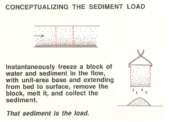
First you must be clear on the distinction between the sediment load and the sediment transport rate. Recall from Chapter 10 that the load is all of the sediment that is being moved by the flow at a given time. Figure \(\PageIndex{1}\) shows how to conceptualize the sediment load. In Figure \(\PageIndex{1}\), you can imagine somehow freezing a block of the flow that contains both water and particulate sediment, and then melting the block to collect the sediment in the block. That sediment is the load. You can think of the sediment load as the depth-integrated sediment mass above a unit area of the sediment bed:
\[L = \text{sediment load} = \int_{0}^{d} c(y) d y\]
where \(c\) is the local time-average sediment concentration. Then the average concentration of transported sediment, \(C\), is equal to \(L/d\).
Just as a review of what was said about the sediment load back in Chapter 10, here are some points or comments about the sediment load:
- There is no fundamental break between the bed load and the suspended load.
- For a given particle that is susceptible to suspension in a given flow, the particle at various times might be traveling as either bed load or as suspended load, or it might temporarily be at rest on the bed surface or within the active layer.
- The ranges of particle size for the bed load and the suspended load in a given flow overlap.
- The suspended bed-material load is not really “suspended”; it is merely traveling, temporarily, in the turbulent flow above the bed.
- The bed-load layer is thin relative to the suspended-load layer.
- The bed-load layer is the lower boundary condition of the suspended-load layer.
- The sediment concentration in the bed-load layer is ordinarily much greater than that in the suspended-load layer.
The Sediment Transport Rate
The sediment transport rate is commonly denoted by \(Q_{s}\). What is more useful, however, and what you are likely to encounter if you have to deal with sediment transport, is the sediment transport rate per unit width of the flow. That is called the unit sediment transport rate; it is often denoted by \(q_{s}\). Think in terms of a vertical slice of the flow, with unit width and oriented parallel to the flow. Which you use depends upon whether you are interested in how much sediment the entire flow carries \((Q_{s})\) or in the inherent intensity of the sediment transport \((q_{s})\).
Below are descriptions of three ways of conceptualizing the sediment transport rate. Each represents, in principle although not necessarily in practice, a way of measuring the sediment transport rate.
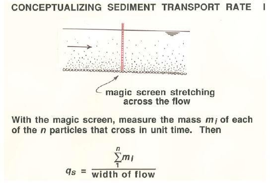
The magic screen: Obtain a magic screen, which, when installed across the flow, allows you to measure the mass \(m_{i}\) of each of the \(n\) particles that pass across the screen in unit time (Figure \(\PageIndex{2}\)). Then
\[q_{s} = \dfrac{ \displaystyle \sum_{1}^{n} m_{i} } { \text{width of flow}}\]
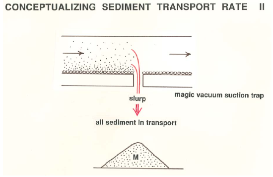
The magic vacuum suction trap: Install a slot, across the entire width of the flow, that allows you to remove all of the particles, both bed load and suspended load, that pass across the cross section of the flow above the slot (Figure \(\PageIndex{3}\)). Think in terms of a magic vacuum cleaner that sucks all of the sediment particles out of the flow and into the trap. (In real life, that would not be extraordinarily difficult for the bed load but virtually impossible for the suspended load.) Suppose that you thereby extract a mass \(M\) of sediment that would have been transported across the location of the cross section in an interval of time \(T\). Then the unit sediment transport rate \(q_{s}\) would be equal to \(M/T\) divided by the width of the flow.
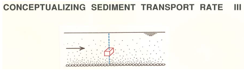
Depth-integrated sampling: (Figure \(\PageIndex{4}\)) Along a vertical in the flow, measure the downstream component of velocity \(v_{i}\) of all of the particles in a tiny imaginary cube in the flow, with volume \(V\), at a given instant. Then multiply \(v_{i}\) by the mass \(m_{i}\) of the particle, and sum over all \(n\) particles found. Divide the result by \(V\) to obtain the transport rate per unit area, and integrate the result over flow depth on a vertical traverse. That give you \(q_{s}\) for that cross-stream position in the flow.
It is notoriously difficult to measure the sediment transport rate, even in controlled settings in laboratory flumes. In a flume, if only bed load is being transported, you can arrange a sediment trap in the form of a narrow slot extending across the entire channel, transverse to the flow direction. Provided that the width of the trap is at least as great as the longest excursions of bed-load particles, all of the bed load falls into the trap, to be collected and weighed. A warning is in order, however: the sampling time must short enough that the deficit in transport does not propagate, by recirculation of the sediment, back to the trap.
In a small stream you can catch the passing bed load by building a dam across the flow, and catch the load in a basket under the overfall across the dam. the problem is that in building the dam you are changing the nature of the stream and its sediment transport for some distance upstream of the dam.
Various kinds of portable bed-load traps have been devised and are in common use. Generally they consist of a receptacle that is open to the flow on the upstream side and screened to pass the water, but catch the sediment, on the downstream side. They are placed on the sediment bed for a time sufficient to catch a measurable quantity of the passing bed load. No matter how well designed, however, such traps distort the flow in their vicinity to a certain extent, and also, if there are rugged bed forms like ripple or dunes on the bed, then the catch depends strongly upon where the trap is placed relative to the crests and troughs of the bed forms.
Measuring the suspended load is a simpler matter, at least in principle. What is commonly done is to trap a volume of passing flow, which contains the suspended load at that particular height above the bed, and combine that with the mean flow velocity at the given level to obtain the proportion of the entire sediment transport rate associated with a narrow interval of the flow depth. If that is done at a large number of heights above the bed, the combined result is a good measure of the suspended-load transport rate. (This is akin to the procedure outlined in the section on depth-integrated sampling, above.)
What is the Relationship between the Sediment Load and the Sediment Transport Rate?
Here is a question for you to ponder. Look back at Figure \(\PageIndex{1}\) and think about the particle size distribution you would find in the pile of sediment that you obtained by melting that instantaneously frozen block of the flow. Now look back at Figure \(\PageIndex{3}\) and think about the particle size distribution you would measure in the pile of sediment you obtained by magically vacuuming out all of the sediment passing by the location of the slot trap. Would those two size distributions be the same or different?
Just a moment’s reflection should convince you that the two distributions would be the same if and only if the transport velocities of each of the particle size fractions in the sediment are the same. If they are not the same— and in general they are not the same, because, at least to a certain extent (we will look at that in more detail in Chapter 3), the coarser fractions tend to move more slowly than the finer fractions—then the particle size distributions will be different in the two cases. That highlights the fundamental difference between the sediment load and the sediment transport rate.