12.2: Unidirectional-Flow Bed Configurations

Introduction

Bed configurations made by unidirectional flows have been studied more than those made by oscillatory flows and combined flows. They are formed in rivers and in shallow marine environments with strong currents, and also in engineering flows like outdoor canals and channels of various kinds, as well as in pipes and conduits carrying granular materials.

In shallow marine environments, even symmetrically reversing tidal currents produce bed forms that look much like those in truly unidirectional flows, presumably because the current in each direction flows for a long enough time for the bed to respond to what it feels as a unidirectional flow. In asymmetrical tidal currents, the bed forms show net movement and asymmetry in the direction of the stronger flow, but they suffer interesting modifications by the weaker flow in the other direction.

A Flume Experiment on Unidirectional-Flow Bed Configurations

To get an idea of the bed configurations produced by a steady uniform flow of water over a sand bed, and the succession of different kinds of bed configurations that appear as the flow strength is increased, imagine making a series of exploratory flume experiments on sand with a mean size between \(0.2\) \(\mathrm{mm}\) and \(0.5\) \(\mathrm{mm}\).

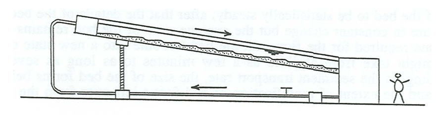
Build a large open channel consisting of wood or metal, with a rectangular cross section (Figure \(\PageIndex{1}\)). The channel might be about one meter wide and a few tens of meters long. Install a pump and some piping to take the water from the downstream end and recirculate it to the upstream end of the channel. You might mount the whole channel on a set of screw jacks near the upstream end, so that you can change the slope of the channel easily, but this is not really necessary. It would also be nice to make at least one sidewall of the channel out of glass or transparent plastic, for good viewing of the bed configurations.

Figure \(\PageIndex{1}\): A home-made flume for studying bed configurations in unidirectional flow.

Place a thick layer of sand on the bottom of the channel and then pass a series of steady and uniform flows over it. Arrange each run to have the same mean flow depth (as great as the flume will allow, ideally at least a large fraction of a meter, but a decimeter or two would suffice) and increase the mean flow velocity slightly from run to run.

In each run, let the flow interact with the bed long enough for the state of the bed to be statistically steady or unchanging. After that time the details of the bed configuration change constantly but the average state of the bed remains the same. The time required for the flow and the bed to come into a new state of equilibrium might be as little as a few minutes or as long as several days, depending on the sediment transport rate, the size of the bed forms that develop, and the extent of modification of bed forms that remained from the preceding run.

You could speed the attainment of equilibrium somewhat by continually adjusting the slope of the channel to maintain uniform flow as the bed roughness changes (the rougher the bed, the steeper the water-surface slope for a given water discharge), but these adjustments are not necessary, because the flow itself adjusts the bed for uniform flow by erosion at one end and deposition at the other.

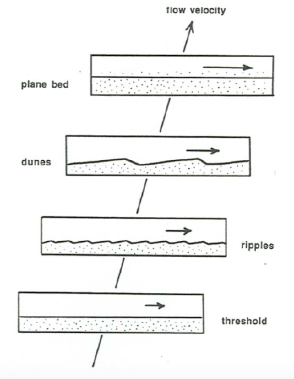
If you are impatient for results, the way to make bed forms develop most rapidly is to start with an irregular sediment bed, but it is more instructive to start with a planar bed. (You can easily arrange a planar bed by passing a straight horizontal scraper blade along the bed. If you mount the blade on a carriage that slides on the straight upper edges of the flume walls, with a little care you obtain a beautifully planar bed.) Now turn the pump on and gradually increase the flow velocity.

Figure \(\PageIndex{2}\): The sequence of bed phases with increasing flow velocity at a given flow depth, for medium sand.

Ripples:

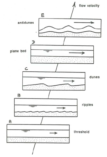
After you exceed threshold conditions (Figure \(\PageIndex{2}\)A), wait for a short time, and the flow will build very small irregularities at random points on the bed, not more than several grain diameters high, from which small ripples develop spontaneously.

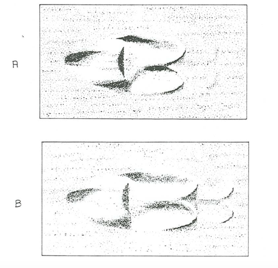
You can help bed forms to develop on the planar bed by poking your finger into the bed at some point to localize the first appearance of bed forms. The flow soon transforms the little mound you made with your finger into a flow-molded bed form. The flow disturbance caused by this bed form scours the bed just downstream, and piles up enough sediment for another bed form to be produced, and so on until a beautiful widening train of downstream-growing bed forms is formed (Figure \(\PageIndex{3}\)). Trains of bed forms like this, starting from various points on the bed, soon join together and pass through a complicated stage of development, finally to become a fully developed bed configuration (Figure \(\PageIndex{2}\)B). The stronger the grain transport, the sooner the bed forms appear, and the faster they approach equilibrium. These bed forms, which I will later classify as ripples, show generally triangular shapes in cross sections parallel to the flow.

Figure \(\PageIndex{3}\): Two stages in the development of a train of ripples from a planar sand bed. Flow is from left to right, and light is from the upper left. The view is straight down on the sand bed. The depression in the left part of the pictures was made by dragging a rod along the bed. The mound thus produced was modified by the flow to become a ripple. (From photographs similar to those shown in Southard and Dingler, 1971.)

At this point I should introduce some terms for the geometry of ripples and other bed forms of similar shape; see Figure \(\PageIndex{4}\). The region around the highest point on the ripple profile is the crest, and the region around the lowest point is the trough. The upstream-facing surface of the ripple, extending from a trough to the next crest downstream, is the stoss surface, and the downstream- facing surface, extending from a crest to the next trough downstream, is the lee surface. A well defined and nearly planar segment of the lee surface, called the slip face, is usually a prominent part of the profile. The top of the slip face is marked by a sharp break in slope called the brink. There is often but not always a break in slope at the base of the slip face also. The top of the slip face is not always the highest point on the profile, and the base of the slip face is not always the lowest point on the profile.

Figure \(\PageIndex{4}\): Terminology for ripple geometry in flow-parallel profile.

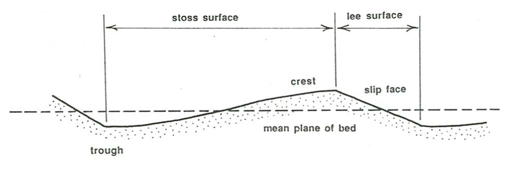
The stoss surfaces of ripples are gently sloping, usually less than about \(10^{\prime}\) relative to the mean plane of the bed, and their lee surfaces are steeper, usually at or not much less than the angle of repose of the granular material in water. Crests and troughs are oriented dominantly transverse to the mean flow but are irregular in detail in height and arrangement. The average spacing of ripples is of the order of \(10–20\) \(\mathrm{cm}\), and the average height is a few centimeters. The ripples move downstream, at speeds orders of magnitude slower than the flow itself, by erosion of sediment from the stoss surface and deposition of sediment on the lee surface.

The field of ripples is commonly three-dimensional, rather than two-dimensional as it would be if the ripples were regular and straight-crested. (This terminology has the potential to be confusing. It is common in fluid dynamics to apply the term two-dimensional to any feature that looks the same in all flow- parallel cross sections. That is true for perfectly regular ripples, with straight, flow-normal crests and troughs that are of the same height all along the ripple.) Most current ripples show great variability in their pattern of crests and troughs, as well as in crest heights and trough depths.

Dunes:

At a flow velocity that is a moderate fraction of a meter per second, ripples are replaced by larger bed forms usually called dunes (Figure \(\PageIndex{2}\)C). Dunes are fairly similar to ripples in geometry and movement, but they are at least an order of magnitude larger. The transition from ripples to dunes is complete over a narrow range of only a few centimeters per second in flow velocity. Within this transition the bed geometry is complicated: the ripples become slightly larger, with poorly defined larger forms intermingled, and then abruptly the larger forms become better organized and dominate the smaller forms. With increasing flow velocity, more and more sediment is transported over the dunes as suspended load. If your flume is large enough, the dunes become large enough under some conditions of sand size and flow velocity for smaller dunes to be superimposed on larger dunes.

Plane Bed:

With further increase in flow velocity the dunes become lower and more rounded, over a fairly wide interval of flow velocity, until finally they disappear entirely, giving way to a planar bed surface over which abundant suspended load as well as bed load is transported (Figure \(\PageIndex{2}\)D). Judging from the appearance of the bed after the flow is abruptly brought to a stop, the transport surface is very nearly planar, with relief no greater than a few grain diameters, although this subtle relief, reflecting the existence and movement of very low-relief bed forms, is thought by some to be responsible for the generation of planar lamination under conditions of net aggradation of the bed (see Chapter 16). Because the bed is obscured by abundant bed load and suspended load, it is difficult to observe the mode of grain transport over the planar bed except through the sidewall of the flume.

Antidunes:

As the flow velocity is increased still further, subdued standing waves appear on the water surface, and the resulting pattern of higher and lower near-bed flow velocity causes the bed to be molded correspondingly into a train of waves that are in phase with the water-surface waves. Under certain conditions these coupled bed waves and surface waves increase in amplitude and become unstable: they move slowly upstream and at the same time grow in amplitude, until they become so steep that they break abruptly, throwing much sediment into suspension (Figure \(\PageIndex{2}\)E). The bed and the water surface then revert to a planar or nearly planar condition, whereupon the waves build again and the cycle is repeated. Because of their upstream movement these forms are called antidunes, so named by G.K. Gilbert (1914) in his pioneering flume experiments on sediment transport and bed configurations.

In an approximate way, the condition for development of antidunes is that the upstream speed of propagation of surface water waves is about the same as the mean velocity of flow, so that the surface water waves have only a small speed relative to the channel bottom. The speed of shallow-water surface waves is well known to be \((g d)^{1 / 2}\) (see Chapter 6), where \(g\) is the acceleration of gravity and \(d\) is the water depth. The condition for development of antidunes is therefore

\[U \approx(g d)^{1 / 2} \label{12.1} \]

or, dividing both sides by the right side to make the terms dimensionless,

\[\frac{U}{(g d)^{1 / 2}} \approx 1 \label{12.2} \]

So conditions are favorable for the development of antidunes when the mean-flow Froude number approaches one. Of course, there must be an underlying instability in the first place to make the antidunes grow in amplitude when in- phase bed waves develop under the water-surface waves.

An instructive variation on your exploratory flume experiment is to increase the flow depth by a factor of two and cover the entire flow with a rigid planar sheet parallel to the mean plane of the bed. The flow structure in the lower half of the closed duct formed in this way is very nearly the same as that in the original open-channel flow (before surface waves set in), except for some differences in the largest-scale eddies in the outer layer owing to the possibility of large eddies making their way across the center plane of the flow, in the case of the closed duct. Now make the same sequence of runs with the top cover in place. You would find the same succession of bed configurations (Figure \(\PageIndex{5}\)) except for one major difference: standing waves and antidunes would not appear, and plane-bed transport would be observed up to indefinitely high flow velocities. This demonstrates that the dynamics of antidunes is unrelated to the dynamics of ripples, dunes, and plane bed: antidunes are dependent upon the presence of the free surface, whereas ripples and dunes are independent of the presence of the free surface.

Figure \(\PageIndex{5}\): Sequence of bed phases as a function of flow velocity over medium sand in a closed conduit.

Dimensional Analysis

Now for a list of the most important variables associated with the fluid, the sediment, and the flow that define the bed state. Once we know the important variables, we can then develop a useful corresponding set of dimensionless variables and plot the positions of bed states observed in the laboratory and in natural flows in a graph with these dimensionless variables along the axes, to identify the fields or regions of existence or stability of the various bed phases. Although that does not address the dynamics behind the various bed phases—a fascinating and complicated matter, about which the last word is nowhere near having been said (see a later section in this chapter)—it provides a useful basis for paleoflow interpretations on the part of sedimentary geologists who work with the ancient sedimentary record, because the various bed configurations are commonly preserved in the record at least partly intact.

As is usual for work with real sediments in nature, even for equilibrium bed states in steady flows the number of variables is depressingly infinite, because an infinite number of variables are needed to describe the joint probability distribution of sediment density, grain size, and grain shape that is associated with any natural sediment. To obtain useful results we have to make some simplifying assumptions. We will assume that the sediment has only a single density and fairly equant particle shape, is subangular to subrounded rather than highly angular or perfectly well rounded, and is moderately well sorted but not unisize. Those assumptions might seem overly restrictive, but they describe most natural sands and fine gravels rather well: most natural sediments have densities not much different from that of quartz and are of approximately equant grain shape. Then the sediment can be characterized fairly well by just the average size \(D\) and the density \(\rho_{s}\). Ignoring the size distribution is not as good an assumption; we should include the sorting \(\sigma\) in the analysis, but few studies have been made on the effect of sorting on bed configuration. The submerged weight per unit volume \(\gamma^{\prime}\) of the sediment must be included in addition to \(\rho_{s}\) to take account of particle weight as well as particle inertia.

As usual, \(\rho\) and \(\mu\) are needed to characterize the fluid. Two variables are needed to describe the flow: a flow-strength variable, and the flow depth \(d\). Keeping in mind the discussion of flow variables in Chapter 8, we will first use \(U\), which will lead to an unambiguous description in a three-dimensional graph, and then \(\tau_{\text{o}}\), which will lead to a two-dimensional graph with considerable overlapping of phase fields, although we will see that with an appropriate method for drag partition, to separate the skin friction from the total bed shear stress, a much better two-dimensional representation is possible.

Using first \(U\) as the flow-strength variable,

\[\text{bed state} =f\left(U, d, D, \rho, \mu, \gamma^{\prime}, \rho_{s}\right) \label{12.3} \]

By dimensional analysis the seven variables chosen in an earlier section as being the most natural in characterizing the bed state can be grouped into four dimensionless variables that equally well characterize the bed state, in the sense that to every combination of the four dimensionless variables there is one and only one dimensionless bed state. Many such sets of dimensionless variables, all equivalent, are possible. Perhaps the simplest set, and certainly the most meaningful in terms of the physics of the flow, is the mean-flow Reynolds number \(\rho U d / \mu\), a mean-flow Froude number \(\rho^{1 / 2} U /\left(\gamma^{\prime} d\right)^{1 / 2}\) written using \(\gamma^{\prime}\), the relative roughness \(d/D\), and the density ratio \(\rho_{s}/\rho\). Another set, more useful sedimentologically in that it segregates \(U\), \(d\), and \(D\) into separate variables (Southard 1971; Harms et al. 1982; Southard and Boguchwal 1990), is

\[\begin{array} \align
\text{Dimensionless flow depth } d^{o}=d\left(\rho \gamma^{\prime} / \mu^{2}\right)^{1 / 3} \\
\text{Dimensionless flow velocity } U^{o}=U\left(\rho^{2} / \mu \gamma^{\prime}\right)^{1 / 3} \\
\text{Dimensionless sediment size } D^{o}=D\left(\rho \gamma^{\prime} / \mu^{2}\right)^{1 / 3} \\
\text{Density ratio } \rho_{s} / \rho \label{12.4} \end{array} \]

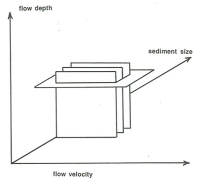
For a given density ratio \(\rho_{s}/\rho\), data on bed states obtained for equilibrium flume runs in steady uniform flow and for field observations in flows thought to be reasonable approximations to steady uniform flow can be plotted in a three-dimensional graph with \(d^{\text{o}}\), \(U^{\text{o}}\), and \(D^{\text{o}}\) along the axes (Figure \(\PageIndex{6}\)). I will call this three-dimensional graph the dimensionless depth–velocity–size diagram. Each bed state that is observed in a flume or in a natural flow can be viewed as one of an infinite number of realizations of a single dimensionless bed state. The corresponding dimensionless depth \(d^{\text{o}}\), dimensionless velocity \(U^{\text{o}}\), and dimensionless sediment size \(D^{\text{o}}\) for that dimensionless bed state can be computed from the given data on \(d\), \(U\), \(D\), \(\rho\), and \(\mu\) and plotted in the graph. The stability fields for the various bed phases occupy certain volumes (three-dimensional regions) in this graph, and the volumes should fill space exhaustively and non-overlappingly. Boundaries between bed phases are three-dimensional surfaces or transitional zones. The graph has to be in three dimensions, but you can see its nature fairly well by making two-dimensional sections through it. Such a graph is loosely analogous to the phase diagrams that petrologists use to represent the thermodynamic equilibrium of mineral phases. Bed-phase stability graphs are a good way of systematizing and unifying disparate data on bed states in a wide variety of flows and sediments.

Figure \(\PageIndex{6}\): The depth–velocity–size diagram for unidirectional-flow bed phases, showing three depth–velocity sections and one velocity–size section.

By virtue of the role of fluid density and fluid viscosity in the dimensional analysis on which the dimensionless variables in Equations \ref{12.4} are based, the dimensionless depth–velocity–size diagram is implicitly standardized for water temperature. It is therefore possible to label the axes of the graph in an alternative way by using depths, velocities, and sizes referred to some arbitrary hypothetical water temperature. In compiling literature data for a depth-velocity-size diagram, I chose a reference temperature of \(10^{\circ}\mathrm{C}\) as being reasonably representative of a wide range of natural subaqueous environments with flow- generated bed configurations in sands; otherwise there is nothing special about it. Using Equations \ref{12.4} I computed from the original data the values of the \(10^{\circ}\mathrm{C}\) depth \(d_{10}\), the \(10^{\circ}\mathrm{C}\) velocity \(U_{10}\), and the \(10^{\circ}\mathrm{C}\) size D10 for a flow of \(10^{\circ}\mathrm{C}\) water dynamically equivalent to the actual flow, in the sense that it corresponds to the same set of values of \(d^{\text{o}}\), \(U^{\text{o}}\), and \(D^{\text{o}}\). This is easily done (Southard and Boguchwal, 1990) for each variable by formulating the dimensionless value both from the given conditions and from the \(10^{\circ}\mathrm{C}\) conditions, setting the two equal,

\[\begin{array}\align d^{o}=d\left(\frac{\rho\gamma^{\prime}}{\mu^{2}}\right)^{1/3}=d_{10}\left(\frac{\rho_{10}\gamma^{\prime}_{10}}{\mu_{10}^{2}}\right)^{1/3}\\U^{o}=U\left(\frac{\rho^{2}}{\mu\gamma^{\prime}}\right)^{1/3}=U_{10}\left(\frac{\rho_{10}^{2}}{\mu_{10} \gamma^{\prime}_{10}}\right)^{1/3} \\\mathrm{D}^{\mathrm{o}}=d\left(\frac{\rho \gamma^{\prime}}{\mu^{2}}\right)^{1 / 3}=D_{10}\left(\frac{\rho_{10} \gamma^{\prime}_{10}}{\mu_{10}^{2}}\right)^{1/3} \label{12.5} \end{array}\]

and then solving for the \(10^{\circ}\mathrm{C}\) value on the assumption that the slight variation of \(\rho\) with temperature can be neglected (the error being by a factor of only \(1.003\) even for \(30^{\prime}\) water):

\[\begin{array} \align
d_{10}=d\left(\frac{\mu_{10}}{\mu}\right)^{2 / 3}\\U_{10}=U\left(\frac{\mu_{10}}{\mu}\right)^{1 / 3}\\D_{10}=D\left(\frac{\mu_{10}}{\mu}\right)^{2 / 3} \label{12.6} \end{array}\]

In the rest of this chapter, depth, velocity, and sediment size referred to \(10^{\circ}\mathrm{C}\) water temperature in this way are called \(10^{\circ}\mathrm{C}\)-equivalent depth, velocity, and sediment size. Note in Equations \ref{12.5} and \ref{12.6} that because the factor in parentheses on the right side of the equations is raised to the \(2/3\) power for \(d\) and \(D\) but to the \(1/3\) power for \(U\), a change in water temperature and therefore \(\mu/\rho\) produces a greater change in effective flow depth and sediment size than in effective flow velocity.

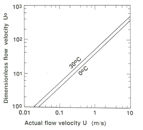
The dimensionless depth–velocity–size diagram presented in a later section from literature data was drawn by computing \(d^{\text{o}}\), \(U^{\text{o}}\), and \(D^{\text{o}}\) for all the data points and plotting those points in a three-dimensional graph with \(d^{\text{o}}\), \(U^{\text{o}}\), and \(D^{\text{o}}\) along the axes. But then the three axes were converted to the \(10^{\circ}\mathrm{C}\)-equivalent quantities \(d_{10}\), \(U_{10}\), and \(D_{10}\) by the procedure outlined above. The interior of the graph remains unchanged, but the graph becomes more useful by providing a concrete representation of depths, velocities, and sediment sizes. The values of \(d^{\text{o}}\), \(U^{\text{o}}\), and \(D^{\text{o}}\) associated with any point in the graph can be obtained using Equations \ref{12.5}. Figure \(\PageIndex{7}\) allows easy conversion between actual values of depth, velocity, and sediment size and dimensionless depth, velocity, and sediment size for two water temperatures, \(0^{\prime}\mathrm{C}\) and \(30^{\prime}\mathrm{C}\).

Figure \(\PageIndex{7}\): Graph for converting between actual flow depth, flow velocity, and particle size, and dimensionless flow depth, flow velocity, and particle size.

If you want to use the dimensionless depth–velocity–size diagram to find the depth, velocity, and size of a bed state at some water temperature other than \(10^{\prime}\mathrm{C}\) that corresponds to a certain point (i.e., a certain dimensionless bed state) in the diagram, you have to use Equations \ref{12.6} in reverse:

\[\begin{array} \align
d=d_{10}\left(\frac{\mu}{\mu_{10}}\right)^{2 / 3}\\U=U_{10}\left(\frac{\mu}{\mu_{10}}\right)^{1 / 3}\\D=D_{10}\left(\frac{\mu}{\mu_{10}}\right)^{2 / 3} \label{12.7} \end{array}\]

Because the particular bed state and the corresponding hypothetical (10^{\prime}\mathrm{C}\) bed state are rigorously similar (geometrically, kinematically, and dynamically), dependent variables with the dimensions of length, like bed-form height or spacing, are in the same ratio between the two states as \(d/d_{10}\) or \(D/D_{10}\), found from Equations \ref{12.5}, \ref{12.6}, or \ref{12.7} to be

\[\frac{d}{d_{10}}=\left(\frac{\mu}{\mu_{10}}\right)^{2 / 3} \label{12.8} \]

and dependent variables with the dimensions of velocity, like the speed of bed-form movement, are in the same ratio between the two states as \(U/U_{10}\), found likewise from Equations \ref{12.5}, \ref{12.6}, or \ref{12.7} to be

\[\frac{U}{U_{10}}=\left(\frac{\mu}{\mu_{10}}\right)^{1 / 3} \label{12.9} \]

It is difficult for the mind to translate values for dimensionless flow depth, flow velocity, and sediment size into real combinations of flow and sediment. In water flows on the Earth’s surface, with water temperatures from \(0^{\circ}\mathrm{C}\) to \(30^{\circ}\mathrm{C}\) and a range of actual flow depths from \(0.01\) \(\mathrm{m}\) to \(10\) \(\mathrm{m}\), dimensionless flow depth ranges from about \(102\) to almost \(106\). Likewise, in the same range of water temperature, for actual flow velocities from \(0.1\) \(\mathrm{m/s}\) to a few meters per second, dimensionless flow velocity ranges from about \(5\) to about \(150\), and for actual sediment sizes from a few hundredths of a millimeter to a few centimeters, dimensionless sediment size ranges from about \(0.5\) to about \(750\).

Hydraulic Relationships

Depth-Velocity-Size Diagram

Figure \(\PageIndex{8}\): Bed phases in graphs of mean flow depth vs. mean flow

Figure \(\PageIndex{8}\).

Figure \(\PageIndex{10}\): Bed phases in a graph of mean flow velocity vs. mean sediment size, for a mean flow depth of \(0.25–0.40\) \(\mathrm{m}\).

Figure \(\PageIndex{10}\).

Figures \(\PageIndex{8}\), \(\PageIndex{9}\), \(\PageIndex{10}\), and \(\PageIndex{11}\) show what the depth–velocity–size diagram for quartz sand in water looks like, on the basis of laboratory experiments made by many investigators. The experiments have been made mainly at flow depths less than a meter. It is much more difficult to obtain data points from deeper natural flows, and none are included in these figures; see below for further discussion of bed configurations in deeper flow depths.

I have labeled the axes in Figures \(\PageIndex{8}\) through \(\PageIndex{11}\) not with the dimensionless variables but with the actual values of flow velocity \(U\), flow depth \(d\), and sediment size \(D\) that correspond to the respective dimensionless variables for an arbitrary reference water temperature of \(10^{\circ}\mathrm{C}\). This provides a concrete feeling for flow and sediment conditions while preserving the interior features of the dimensionless graph. Ignoring the water temperature would lead to considerable scatter in the data points, and would obscure the strong regularities shown by the dimensionless diagram.

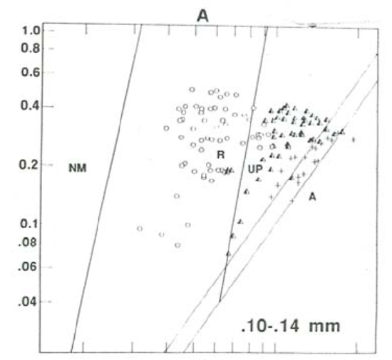
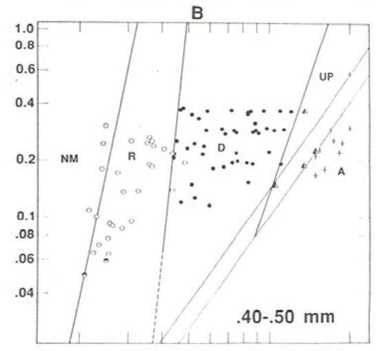
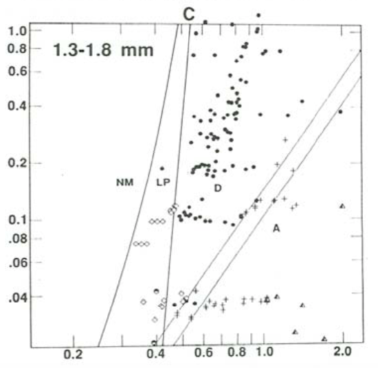
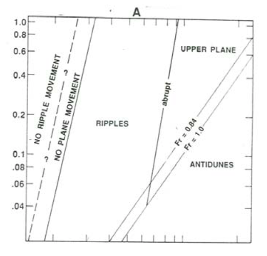
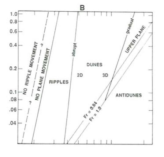
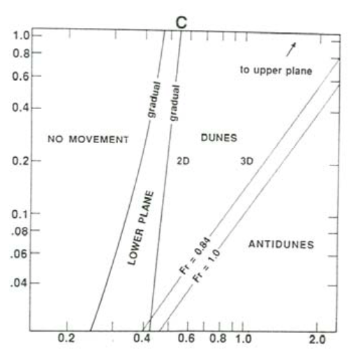
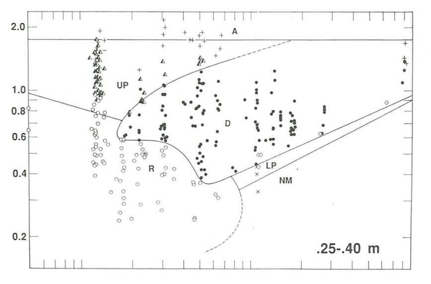
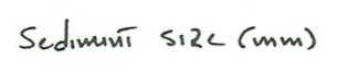
Figures \(\PageIndex{8}\) and \(\PageIndex{9}\) show three depth–velocity sections for sediment sizes of \(0.10–0.14\) \(\mathrm{mm}\), \(0.40–0.50\) \(\mathrm{mm}\), and \(1.30–1.80\) \(\mathrm{mm}\). Figure \(\PageIndex{8}\) shows data points from many experimental studies, and Figure \(\PageIndex{9}\) is a schematic version of Figure \(\PageIndex{8}\). Figures \(\PageIndex{10}\) and \(\PageIndex{11}\) show a velocity–size section for a flow depth of \(0.25–0.40\) \(\mathrm{m}\). Figure \(\PageIndex{10}\) shows data points, and Figure \(\PageIndex{11}\) is a schematic version. Figures \(\PageIndex{8}\) through \(\PageIndex{11}\) are from Boguchwal and Southard (1990).

The section for \(0.10–0.14\) \(\mathrm{mm}\) sand (Figures \(\PageIndex{8}\)A, \(\PageIndex{9}\)A) shows fields only for ripples, upper-regime plane bed, and antidunes. All the boundaries here and in the other two graphs in Figures \(\PageIndex{8}\) and \(\PageIndex{9}\) slope upward to the right. The boundary between ripples and plane bed slopes in that sense because the deeper the flow the greater the velocity needed for a given bed shear stress. The boundary between plane bed and antidunes slopes in that sense because it is well represented by the condition that the Froude number \(U/(gd)^{1/2}\) is equal to one, as discussed above. The latter boundary is shown to truncate the former, because (though data are scanty) as the Froude number approaches one, antidunes develop irrespective of the preexisting configuration. This relation holds true also, and more clearly, for coarser sediments (Figures \(\PageIndex{8}\)B, \(\PageIndex{8}\)C, \(\PageIndex{9}\)B, \(\PageIndex{10}\)C).

Figure \(\PageIndex{8}\)A (and Figure \(\PageIndex{8}\)B, for medium sands, as well) show two kinds of boundary between movement and no movement. To the right is the curve for incipient movement on a plane bed, and to the left is the boundary that defines the minimum velocity needed to maintain preexisting ripples at equilibrium. It is clear that the latter boundary lies to the left of the former, but the existing data are not good enough to define the positions of these boundaries well. (Only the former boundary is shown in Figures \(\PageIndex{8}\)A and \(\PageIndex{9}\)B.)

The section for \(0.40–0.50\) \(\mathrm{mm}\) sand (Figures \(\PageIndex{8}\)B, \(\PageIndex{9}\)B) shows an additional field for dunes between the fields for ripples and for plane bed. The boundary between dunes and plane bed clearly slopes less steeply than the boundary between ripples and dunes. For depths less than about \(0.05\) \(\mathrm{m}\) it is difficult to differentiate between ripples and dunes, because dunes become severely limited in size by the shallow flow depth. The appearance and expansion of the dune field with increasing sediment size pushes the lower termination of the plane-bed field to greater depths and velocities, nearly out of the range of most flume work. The antidune field truncates not only the ripple field, as with finer sands, but the dune field as well.

In the section for \(1.30–1.80\) \(\mathrm{mm}\) sand (Figures \(\PageIndex{8}\)C, \(\PageIndex{9}\)C), a lower- regime plane bed replaces ripples at low flow velocities. Upper-regime plane bed is still present in the upper right, but few flume data are available. Upper-regime plane beds succeed antidunes with increasing velocity and decreasing depth in the lower right; apparently the bed becomes planar once again as the Froude number becomes sufficiently greater than one. The left-hand boundary in Figures \(\PageIndex{8}\)C and \(\PageIndex{9}\)C represents the threshold for sediment movement on a plane bed. Sections for even greater sediment size are qualitatively similar to the section shown in Figures \(\PageIndex{8}\)C and \(\PageIndex{9}\)C.

In the velocity–size section for flow depths of \(0.25–0.40\) \(\mathrm{m}\) (Figures \(\PageIndex{10}\), \(\PageIndex{11}\)), ripples are the stable bed phase for sediment sizes finer than about \(0.8\) \(\mathrm{mm}\). The range of flow velocity for ripples becomes narrower with increasing sediment size, and the ripple field finally ends against the fields for plane beds with or without sediment movement. Relationships in this region are difficult to study because in these sand sizes and flow velocities a long time is needed for the bed to attain equilibrium. In medium sands ripples give way abruptly to dunes with increasing flow velocity, but, in finer sediment, ripples give way (also abruptly) to plane bed. Although not well constrained, the ripple–plane boundary rises to higher velocities with decreasing sediment size.

Dunes are stable over a wide range of flow velocities in sediments from medium sand to indefinitely coarse gravel. Both the lower and upper boundaries of the dune field rise with increasing flow velocity, and both are gradual transitions rather than sharp breaks. For sediments coarser than about \(0.8\) \(\mathrm{mm}\) there is a narrow field below the dune field for lower-regime plane bed; the lower boundary of this field is represented by the curve for threshold of sediment movement on a plane bed.

There is one triple point among ripples, dunes, and upper plane bed at a sediment size of about \(0.2\) \(\mathrm{mm}\), and another among ripples, dunes and lower plane bed at a sediment size of about \(0.8\) \(\mathrm{mm}\). The coverage of data around these two triple points constrains the bed-phase relationships fairly closely. Between these two triple points the dune field forms a kind of indented salient pointing toward finer sediment sizes. The boundary between ripples and upper plane bed seems to pass beneath the dune field at the upper left triple point to emerge again at coarser sediment size and lower flow velocity as the boundary between ripples and lower plane bed at the lower right triple point.

Other velocity–size sections, for other flow depths, show the same qualitative relationships as Figures \(\PageIndex{10}\) and \(\PageIndex{11}\). With increasing flow depth the lower boundary of the antidune field rises very rapidly, and antidunes are unimportant in flows greater than a few meters deep. All the other boundaries rise more slowly with increasing flow depth. There is also some change in the shape of the dune field with increasing flow depth.

Figure \(\PageIndex{12}\): Schematic depth–velocity–size diagram showing bed-phase stability field for bed phases in steady unidirectional water flows with a wide range of flow depths in flumes and natural environments. (From Rubin and McCulloch, 1980.)

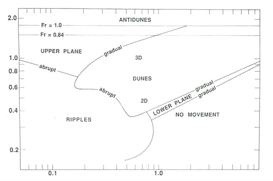
Numerous observations of bed configurations in natural environments in which sands are subjected to fairly steady unidirectional flows indicate that the stability relationships of bed configurations in deeper flows are a straightforward extrapolation of the depth–velocity–size diagram discussed above. Ripples are almost the same in shallow flows and deep flows, but dunes in deep flows are much larger than dunes in shallow flows. Figure \(\PageIndex{12}\), after Rubin and McCulloch (1980), shows an extrapolation of the depth–velocity–size diagram to much greater flow depths based on data from several studies in natural flow environments.

Figures \(\PageIndex{8}\) and \(\PageIndex{10}\) in the depth–velocity–size diagram.

Figures \(\PageIndex{8}\) and \(\PageIndex{10}\) in the depth–velocity–size diagram.

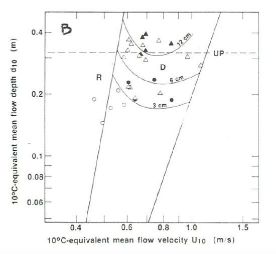
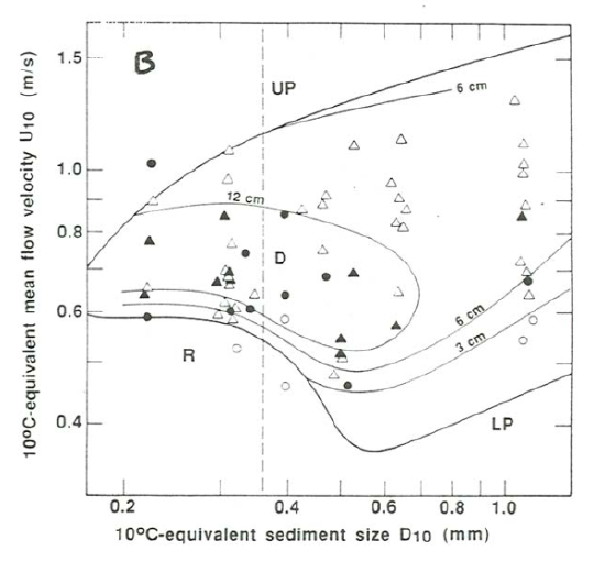
There must be a definite average dune height and spacing associated with each point in the existence field for dunes in the depth–velocity–size diagram. Unfortunately, few experimental studies have reported dune dimensions systematically. Figures \(\PageIndex{13}\) and \(\PageIndex{14}\) make use of data on dune spacings and heights from the best data set, that of Guy et al. (1966), in a crude attempt to contour dune spacings and heights in the depth–velocity–size diagram. Figures \(\PageIndex{13}\)A and \(\PageIndex{13}\)B show contours of dune spacing and height in a depth–velocity section for a sediment size of \(0.30–0.40\) \(\mathrm{mm}\), and Figures \(\PageIndex{14}\)A and \(\PageIndex{14}\)B show contours of dune spacing and height in a velocity–size section for a flow depth of \(0.25–0.40\) \(\mathrm{m}\).

In the depth-velocity section (Fig. \(\PageIndex{13}\)A), dune spacing increases from lower left to upper right, with increasing depth and velocity. In the velocity-size section (Fig. \(\PageIndex{14}\)A), dune spacing increases from lower right to upper left with increasing velocity and decreasing sediment size; the greatest spacings are at the upper-plane-bed boundary and a sediment size of between \(0.2\) and \(0.3\) \(\mathrm{mm}\). Dune height shows a different and more complicated behavior. In the depth–velocity section (Fig. \(\PageIndex{13}\)B), dune height increases monotonically with increasing depth but shows an increase and then a decrease with increasing flow velocity at constant depth. In the velocity–size section (Fig. \(\PageIndex{14}\)B), there is an elongated core of greatest heights extending from near the left-hand extremity of the dune field, at the finest sizes of about \(0.2\) \(\mathrm{mm}\), rightward to sizes of \(0.5\) to \(0.6\) \(\mathrm{mm}\). Heights seem to decrease in all directions from that core, most rapidly with decreasing flow velocity.

The sections in Figures \(\PageIndex{13}\) and \(\PageIndex{14}\) intersect each other at right angles at the dashed line shown on both sections. You have to imagine the contours as cuts through a family of curved surfaces in three dimensions filling the dune field in the depth–velocity–size diagram.

Diagrams with Bed Shear Stress

So far we have looked at the hydraulic relationships of bed phases using the mean flow velocity \(U\) as the flow-strength variable. Most investigators have chosen to use the bed shear stress \(\tau_{\text{o}}\) rather than \(U\). What do the same relationships look like in graphs using the bed shear stress \(\tau_{\text{o}}\)? One thing we can say right away about such graphs is that the effect of flow depth is much less: the effect of the substantial change in velocity with flow depth for a given bed shear stress is no longer relevant, and all that is left is the smaller effect on the bed shear stress of changes in bed-form geometry with flow depth. A single suitably nondimensionalized two-dimensional graph of bed shear stress against sediment size should therefore be expected to represent bed states reasonably well. Simons and Richardson (1966) seem to have been the first to use such a plot, although in the dimensional form of \(\tau_{\text{o}}\) vs. \(D\). A later and more comprehensive of plots of this kind was given by Allen (1982, Vol. 1, p. 339–340), who plots Shields parameter and dimensionless (temperature-standardized) stream power against dimensionless (temperature-standardized) sediment size.

Boundary shear stress can be nondimensionalized in various ways. The conventional way is to form a dimensionless variable containing \(\tau_{\text{o}}\) and \(D\), namely \(\tau_{\mathrm{o}} / \gamma^{\prime} D\), usually called the Shields parameter (see Chapter 9). One can also work with a dimensionless form of the stream power \(\tau_{\text{o}}U\), on the theory that the sediment transport depends most fundamentally upon stream power. Another alternative is \(\tau_{\text{o}}\left(\rho / \gamma^{\prime 2} \mu^{2}\right)^{1 / 3}\), which I call here the dimensionless boundary shear stress \(T^{\text{o}}\). The disadvantage with \(T^{\text{o}}\) is that it does not embody the physics of the phenomenon nearly as well as the Shields parameter, but the advantage is that, when \(T^{\text{o}}\) is used with \(D^{\text{o}}\), \(\tau_{\text{o}}\) and \(D\) do not appear together in the same dimensionless variable. We will work with this last alternative, because it lends itself more directly to temperature standardization, which is important in the range of conditions for which Reynolds-number effects cannot be neglected, and also because sediment-size effects are thereby manifested entirely through the dimensionless sediment size \(D\left(\rho \gamma^{\prime} / \mu^{2}\right)^{1 / 3}\).

Figure \(\PageIndex{15}\): Bed phases in a dimensionless (temperature-standardized) plot of sidewall-corrected bed shear stress vs. sediment size for bed phases. labels for regions: I, no movement on plane bed; II, ripples; III, lower plane bed; IV, dunes; V overlap region of dunes, upper plane bed, and antidunes; VI, overlap region of ripples, upper plane bed, and antidunes; VII overlap region of upper plane bed and antidunes.

Figure \(\PageIndex{15}\).

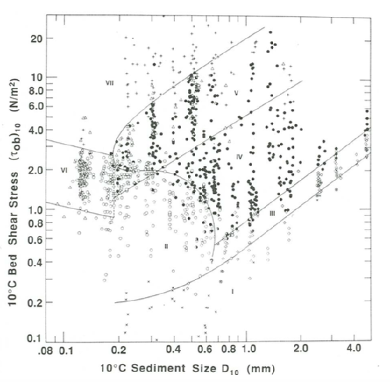
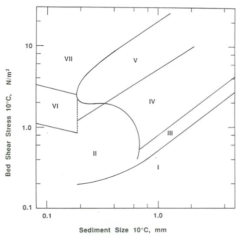
Figure \(\PageIndex{15}\) is a plot of \(T^{\text{o}}\) vs. \(D^{\text{o}}\) showing the stability fields for the various bed phases. The same data sources were used as for the depth–velocity– size graph discussed above, except that fewer studies were used because some studies that reported the mean flow velocity did not report the energy slope, so \(\tau_{\text{o}}\) could not be computed. Only runs made at depths greater than \(0.06\) \(\mathrm{m}\) were used. In all, \(1204\) runs were used. \(10^{\circ}\mathrm{C}\)-equivalent flow depths \(d_{10}\) range from \(0.06\) \(\mathrm{m}\) up to the deepest reported in the sources used, a little greater than \(1\) \(\mathrm{m}\) (by Nordin 1976). Figure \(\PageIndex{16}\) is a schematic version of Figure \(\PageIndex{15}\).

The value of τo for each run was corrected for sidewall effects by the method proposed by Vanoni and Brooks (1957). (For a summary of this method, see Vanoni 1975, p. 152–154.) The result is an estimate of the shear stress \(\tau_{\text{o}b}\) acting on the sediment bed only. Because the bed is always rougher than the sidewalls (except for dynamically smooth flow over a planar granular bed), and the width/depth ratio is never infinite, this estimate of \(\tau_{\text{o}b}\) is always greater than the boundary shear stress averaged over the wetted perimeter of the flow, which is found from the experimental data by use of the resistance equation for steady uniform flow in an open channel, \(\tau_{\text{o}}=\rho g A S / p\), where \(A\) is the cross-sectional area of the flow and \(p\) is the wetted perimeter of the flow. For bed states with rugged flow-transverse bed forms in flows with small width/depth ratios, \(\tau_{\text{o}b}\) can be almost half again as large as \(\tau_{\text{o}}\).

The axes of the graph in Figure \(\PageIndex{15}\) are not labeled with \(T^{\text{o}}\) and \(T^{\text{o}}\) but with \(D_{10}\) and \(\left(\tau_{\mathrm{o}b}\right)_{10}\), the sidewall-corrected bed shear stress standardized to a water temperature of \(10^{\circ}\mathrm{C}\). As with depth, velocity, and size in an earlier section, (\left(\tau_{\mathrm{o}b}\right)_{10}\) is related to (\tau_{\mathrm{o}b}\) by the equation

\[\left(\tau_{\text{o}b}\right)_{10}=\tau_{\text{o}b}\left(\frac{\mu_{10}}{\mu}\right)^{2 / 3} \label{12.10} \]

obtained by equating values of \(T^{\text{o}}\) for \(10^{\circ}\mathrm{C}\) and for the given conditions and solving for \(\left(\tau_{\mathrm{o}b}\right)_{10}\) on the assumption that \(\rho\) and \(\gamma^{\prime}\) do not vary with temperature.

Scatter or overlapping of points for different bed phases is much greater in Figure \(\PageIndex{15}\) than in the various sections through the dimensionless depth– velocity–size diagram, for two main reasons:

1. It is well known that because the form resistance, which is the dominant contribution to the total bed shear stress over rugged flow-transverse bed forms, disappears in the transition from ripples to upper plane bed or from dunes to upper plane bed, the total bed shear stress actually decreases with increasing mean flow velocity in these transitions before it increases again. For that reason, there is a certain range of \(\tau_{\text{o}b}\) for which three different values of \(U\) are possible; see Figure 8.5.1, back in Chapter 8. In a plot of \(\tau_{\text{o}b}\) against \(D\), this means that there is an approximately horizontal band across the graph in which values of \(U\), and thus also their associated bed phases, overlap or fold onto one another. In Figure \(\PageIndex{15}\) this is shown as a field of overlapping dunes, upper plane bed, and antidunes, labeled \(V\), and a field of overlapping ripples, upper plane bed, and antidunes, labeled VI.
2. Accurate measurement of water-surface slope \(S\), and therefore \(\tau_{\text{o}}\), is understandably less accurate than measurement of \(U\): water-surface slopes are small, so long channels and careful surveying are needed, and in any case the slope varies with time around some long-term average as the details of the bed configuration fluctuate, so long time series of \(S\) are needed for good accuracy. These problems with the slope presumably affect all of Figure \(\PageIndex{15}\), but they are noticeable only at bed-phase boundaries that should not be affected by the shear-stress ambiguity noted above, like the boundary between ripples and dunes or the boundary between lower plane bed and dunes.

The effects of data scatter and phase-field overlap make partitioning Figure \(\PageIndex{15}\) into existence fields for the various bed phases not a straightforward matter. The more straightforward results for the depth–velocity–size diagram were used as a guide in developing a rational partition.

Because of the moderate degree of scatter of ripple and dune points, the boundary between ripples (Region II) and dunes (Region IV) can be located only in a general way. The overall shape of the boundary was made qualitatively similar to that in the depth–velocity–size diagram (Figures \(\PageIndex{8}\) through \(\PageIndex{11}\)). It is reasonable to suppose that this boundary continues downward past the question mark and then leftward to define the minimum shear stress for existence of ripples, as in Figures \(\PageIndex{10}\) and \(\PageIndex{11}\). Because few investigators have attempted to identify the weakest flows for which preexisting ripples are maintained as flow strength is very gradually decreased while equilibrium is maintained, existing data are inadequate to define the position of this extension. Either the plane-bed threshold curve is eclipsed by the lower part of the ripple field, as in Figures \(\PageIndex{10}\) and \(\PageIndex{11}\), or the lower boundary of the ripple field is at bed shear stresses entirely above those for the plane-bed threshold curve. The threshold curve itself is not extended leftward because of this uncertainty.

Interpretation of the remaining boundaries is based upon the existence of a minimum sediment size of about \(0.15–0.20\) \(\mathrm{mm}\) for existence of dunes, as shown clearly by left-pointing “nose” of the dune field in the velocity–size sections through the depth–velocity–size diagram together with the effect of the \(\tau_{\text{o}\) ambiguity on the relations among ripples, dunes, and plane beds. As in the velocity–size sections through the depth–velocity–size diagram, the ripple–dune boundary in Figure \(\PageIndex{16}\) is interpreted to pass leftward through an inflection point and then curve upward and again rightward, passing through the sediment-size minimum for dunes, to become the upper limit of dune stability (between Regions V and VII).

Owing to the shear-stress ambiguity there is a substantial range of shear stresses below this upper boundary for dunes for which either dunes or plane bed can exist. The lower limit of this overlap region (Region V) is shown as a straight line sloping downward to the left. Neither the shape nor the position of this line is well constrained by the data. By its nature, this boundary must end leftward at the minimum sediment size for the existence of dunes; it is therefore connected upward to the point of minimum sediment size by a vertical dashed line. In the small unlabeled region with approximately triangular shape (bounded below by this lower limit of upper-plane-bed stability, above by the upper limit of ripple stability, and to the left by the leftward limit of dune stability), ripple and dune points overlap.

To the left of the minimum sediment size for dunes, ripple pass directly into upper plane bed with increasing flow strength, and again there is a broad region of overlap of ripples and upper plane bed (Region VI). In this region the vertical span of the overlap region is about as great as the span of available data, so the two boundaries sloping downward to the right here (the upper showing the maximum shear stresses for existence of ripples, and the lower showing the minimum shear stresses for existence of plane beds) are poorly constrained. The slopes of these lines were chosen only by analogy with that of the boundary between ripples and upper plane bed in the velocity–depth sections of the depth–velocity–size diagram; both their slope and their parallelism are arbitrary.

The upper of these two boundaries, giving the upper limit for ripples, is shown to end at the sediment-size minimum for dunes (i.e., the point of vertical tangent at the leftward extremity of the dune field), although this is not a necessity: the intersection could just as well lie somewhat above or somewhat below that point. In any case, the second of these boundaries, representing the lower limit for existence of upper plane beds, must terminate rightward at the same sediment size—hence the vertical dashed line connecting the two boundaries. Because the intersection should not be expected to be exactly at the minimum sediment size for dunes, this vertical dashed line should actually be at a slightly different and greater sediment size from the vertical dashed line, mentioned above, that connects the two analogous curves for dunes at greater sediment sizes. So there must really be two vertical dashed lines, very close together. Existing data, extensive as they are, are inadequate to locate the two corresponding sediment sizes with certainty, and they are shown as a single vertical dashed line in Figure \(\PageIndex{15}\).

Points for antidunes appear throughout Regions VI and VII and in the upper part of Region V in Figure \(\PageIndex{15}\). Presumably the reason there is no boundary between upper plane bed and antidunes in what is labeled as Region VII in Figure \(\PageIndex{15}\) is that the transition from upper plane bed to antidunes with increasing flow velocity at the flow depths characteristic of many flume experiments takes place at bed shear stresses well below those of Region VII.

The consequences of lumping all flow depths into the single plot represented by Figure \(\PageIndex{15}\) are substantial only for antidunes, because the onset of antidunes depends upon the mean-flow Froude number. Plots of \(\left(\tau_{\text{o}b}\right)_{10}\) vs. \(D_{10}\) for the individual depth categories used in plotting the depth–velocity–size diagram show a systematic, although still scattered, rise in the position of the minimum shear stresses for antidunes as flow depth increases. Other effects of flow depth on the positions of the various boundaries in \(\left(\tau_{\text{o}b}\right)_{10}–D_{10}\) plots are so minor as to be swamped by the data scatter.

Figure \(\PageIndex{15}\). Symbols: solid circles, upper plane bed; bull’s-eye circles, antidunes; open circles, ripples.

Figure \(\PageIndex{17}\).

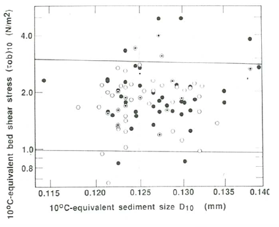
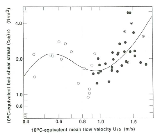
The welter of overlapped points for ripples, upper plane bed, and antidunes for sediment sizes around \(0.12\) \(\mathrm{mm}\), mostly from the work of Willis et al. (1972), is difficult to distinguish in Figure \(\PageIndex{15}\), so all the runs made in that study for which slope was reported are replotted in Figure \(\PageIndex{17}\) with the sediment-size axis stretched relative to the shear-stress axis. The straight lines represent the minimum shear stresses for ripples and the minimum shear stresses for upper plane beds, taken from Figure \(\PageIndex{15}\). The thorough blending of points for the three phases is clear. Figure \(\PageIndex{18}\), a plot of \(10^{\circ}\mathrm{C}\)-equivalent bed shear stress against \(10^{\circ}\mathrm{C}\)-equivalent mean flow velocity for those same points, shows why the points in Figure (\PageIndex{17}\) are so scrambled. Despite the considerable scatter, there clearly is first an increase, then a decrease, and then again an increase in shear stress with increasing velocity, as shown by the curve that represents very approximately the trend of the data points. The range in shear stress between the local minimum and the local maximum in that curve, together with the inevitable scatter in the shear stresses themselves, is sufficient for substantial mixing of the points.

The plot in Figure \(\PageIndex{15}\) could be transformed into a plot of Shields parameter against dimensionless sediment size, or into a plot of dimensionless flow power against dimensionless sediment size (neither of which is shown here), but with no obvious advantages for sedimentological interpretation. These plots would be qualitatively different in certain ways from those presented by Allen (1982) because of the influence of the results from the depth–velocity–size diagram on our method of partitioning Figure \(\PageIndex{15}\).

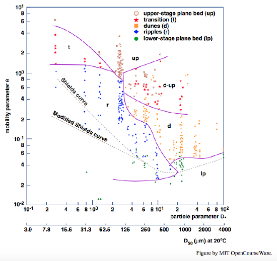
Van den Berg and van Gelder (1993) introduced a bed-phase stability diagram (Figure \(\PageIndex{19}\)) based on boundary shear stress that in large part removes the difficulties discussed above. The horizontal axis is the dimensionless sediment size used above, and the vertical axis is a Shields parameter modified in such a way that the bed shear stress is represented by the part generated by the particle roughness rather than the form drag associated with bed forms. The strategy is to express the bed shear stress in terms of a Chézy coefficient (see Chapter 4) that is a function of the ratio of water depth to \(D_{90}\), the ninetieth-percentile particle size. This largely circumvents the dominance of form drag in the presence of rugged bed forms. You can see from the diagram that there is much less ambiguity in partitioning of existence fields than in Figure \(\PageIndex{15}\), but there is still considerable overlap between dunes and upper plane bed, suggesting that the method for drag partitioning is still less than perfect. Nonetheless, Figure \(\PageIndex{19}\) is a great improvement over earlier existence diagrams based on bed shear stress.

Figure \(\PageIndex{19}\): Existence fields for bed phases in a dimensionless plot of modified Shields parameter vs. dimensionless sediment size. (From van den Berg and van Gelder, 1993.)

Flow Regimes

This is the place to be more specific about the terms lower flow regime and upper flow regime I have used a few times already. Simons and Richardson (1963) proposed that bed phases be classified into a lower flow regime and an upper flow regime on the basis of the transition from the rugged ripple-like bed phases (ripples and dunes) formed at relatively low flow strengths and the less rugged bed phases (upper plane bed and antidunes) formed at high flow strengths (Figure \(\PageIndex{20}\)A). The motivation for this classification was not so much the sharp distinction in bed geometry in itself as the great decrease in flow resistance in passing from the lower flow regime to the upper flow regime. Geologists have found the distinction useful not only in terms of the differing bed geometry but also in terms of the consequent great difference in sedimentary structures produced: with the minor exception of lower-regime plane beds, lower-regime conditions give rise to cross-stratified structures, whereas upper-regime conditions give rise mostly to planar lamination—although antidunes produce cross-stratification as well: see Chapter 15.

Figure \(\PageIndex{10}\)) showing the customary division into an upper flow regime and a lower flow regime based on the transition from ripple and dune bed phases to upper plane bed or antidunes. B) The same velocity–size diagram showing an alternative division into a lower group of bed phases (lower plane bed ripples, dunes, and upper plane bed) whose dynamics are independent of the presence of a free surface and an upper bed phase (antidunes) whose dynamics are dependent upon the presence of a free surface.

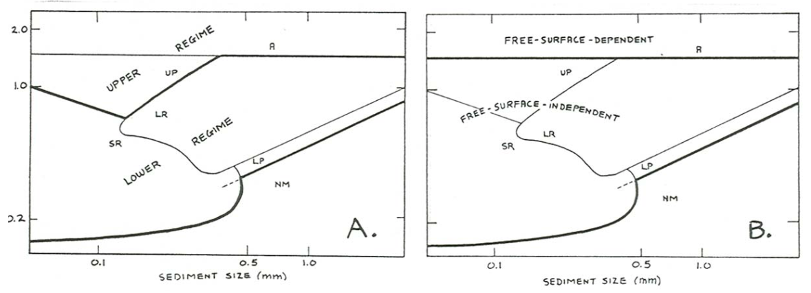
In terms of bed-configuration dynamics, it is also natural to divide bed phases into two groups in a different way on the basis of the importance of a free surface (Figure \(\PageIndex{20}\)B). Ripples, dunes, and plane bed are bed phases whose occurrence is independent of the existence of a free surface: recall that in the exploratory flume experiments described earlier in this chapter the existence of ripples was not affected by placing a board over the water surface. These bed phases could therefore be termed free-surface-independent bed phases. Antidunes, on the other hand, are dependent upon the existence of a free surface, and could therefore be termed a free-surface-dependent bed phase.

Flow Over Ripples and Dunes

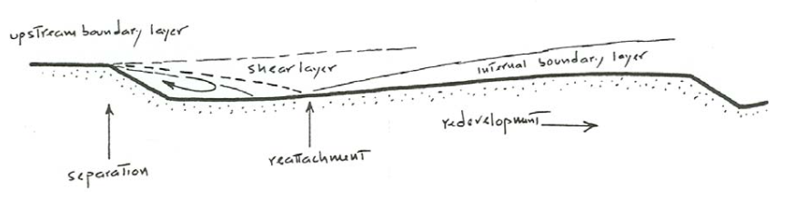
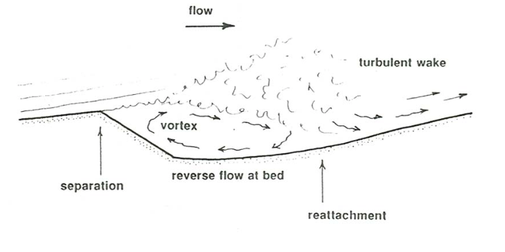
Flow over ripples and dunes is dominated by flow separation, a phenomenon whereby the flow separates from the solid boundary in the region where the boundary curves away from the general upstream flow direction. The general picture of separated flow over a ripple or a dune is shown in Figure \(\PageIndex{21}\), and in more cartoonlike form in Figure \(\PageIndex{22}\). When the flow reaches the crest it continues to move in the same direction rather than bending downward to follow the contour of the bed. Strong turbulence develops along the surface of strong shear, called the shear layer, which represents the contrast between the high velocity in the separated flow and the low velocity in the shelter of the bed form. This turbulence expands both upward and downward, and at some position downstream of the crest the turbulent shear layer meets the sediment bed. The flow is said to reattach to the bed at that point. Downstream of reattachment, the flow near the bed is directed downstream once again. Upstream of reattachment, in what is called the separation vortex, the bed feels a weak flow in the reverse direction.

Figure \(\PageIndex{21}\): Flow structure over ripple or dune bed forms. (Schematic, but not much vertical exaggeration.)

Figure \(\PageIndex{21}\) that is less schematic but has some vertical exaggeration.

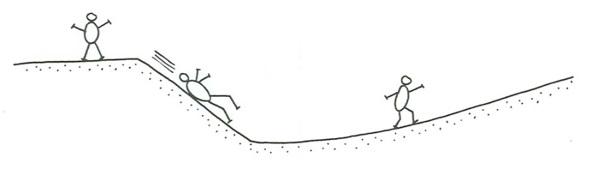
Take a tour of a ripple or dune profile by starting at a crest, sliding down the slip face, and then walking across the trough and up the stoss surface of the next bed form downstream (Figure \(\PageIndex{23}\)). The flow you would feel differs greatly along the profile. With the appropriate equipment you could actually do this on a large dune in a river or a tidal current, or more easily on a subaerial dune when the wind is blowing. Refer to Figures \(\PageIndex{21}\) and \(\PageIndex{22}\) as you read the next paragraph.

Figure \(\PageIndex{23}\): A field trip on a dune.

As you move down the slip face and into the trough you would feel a weak, irregular, eddying current in the opposite direction. Near the reattachment line you would feel the full effect of the turbulence in the shear layer. In the reattachment zone the strong eddies generated in the shear layer impinge upon the bed and flatten out against it to cause temporarily very high local shear stresses. You would feel strong puffs or gusts of flow trying to push you this way and that. But even though the shear stress is high at certain points and certain times, it is nearly zero on the average. As you continue to walk up the slope toward the next crest, the flow velocity and therefore the boundary shear stress would gradually increase, because the flow is crowded upward, but the intensity of the turbulence would lessen.