7.6: Ekman Layers

It might have occurred to you, the perceptive reader, that there has to be something more to the phenomenon of geostrophic motion than what I have shown above—because the air somehow has to get down the pressure gradient, or else the pressure gradients would keep on increasing. (Think back to the convection-cell example I presented earlier.) Somehow there has to be movement of the air across the isobars, as in the more direct flow that would be set up in the absence of rotation.

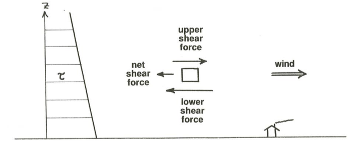
The way out of this dilemma is to include the effect of friction forces in the lowermost part of the atmosphere. Think about the friction forces on a small test parcel of air moving near the ground. The overlying and underlying layers of air exert friction forces on the top and bottom surfaces of the parcel, and these forces are in different directions: the lower layer exerts a force opposite to the direction of motion, and the upper layer exerts a force in the direction of motion. The key point (Figure \(\PageIndex{1}\)) is that the upper of these shear forces is slightly smaller than the lower, because the shear stress decreases upward from a maximum at the ground, just as in open-channel flow we considered in Chapter 4. So the net friction force should act opposite to the direction of motion.

Figure \(\PageIndex{1}\): The net shear force on a parcel of air parcel moving near the Earth’s surface or on a parcel of water moving near the ocean bottom. (The effect of the turning of the flow in the bottom Ekman layer is not taken into account in this approximate sketch; see the section on the bottom Ekman layer in the text for a more realistic account.)

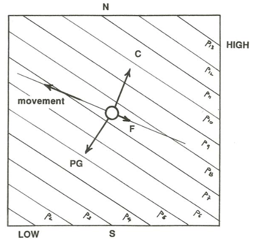
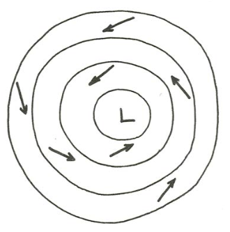
Now a qualitative balance among the three forces (pressure gradient, large; Coriolis, large; friction, small but nonnegligible) shows (Figure \(\PageIndex{2}\)) that the wind blows across the isobars at a small angle from high pressure to low pressure. This you can see clearly on any good weather map (of which the map in Figure \(\PageIndex{3}\) is a cartoon version) drawn for conditions at the surface, where the frictional influence is greatest: the air spirals inward toward the low-pressure area, there to have a small upward component to its motion and then flow outward at high altitudes in compensation for the inflow at low altitudes. The origin of the friction force shown in Figure \(\PageIndex{2}\) is of the same nature as was shown in Figure 7.4.2 for the surface Ekman layer: as the flow turns, the directions, as well as the magnitudes, of the friction forces on the top and on the bottom of a fluid element are slightly different, leading to a net friction force at a large angle to the direction of motion of the element.

Figure \(\PageIndex{2}\): The effect of near-surface friction makes the wind blow across the isobars at a small angle toward lower pressure.

Figure \(\PageIndex{3}\): Cartoon weather map showing a low-pressure area, with winds blowing counterclockwise around the place of lower pressure but with a component spiraling inward across the isobars.

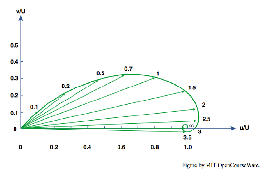
The lowermost layer of the atmosphere or the ocean, adjacent to the land surface in the case of the atmosphere or to the ocean bottom in the case of the ocean, in which the direction of flow turns gradually from the direction of the overlying geostrophic flow, is called the Ekman layer (or the bottom Ekman layer). The mathematical solution for the structure of the Ekman layer was developed by Ekman in 1905. (See Pedlosky, 1979, Chapter 4, for a lucid derivation.) The Ekman layer is the region of the flow in which the frictional effect of the bottom boundary is significant. Downward through the Ekman layer, the magnitude of the velocity decreases from its geostrophic value to zero, by the no-slip condition, at the bottom and the direction of the velocity turns from the geostrophic direction to its maximum deviation at the bottom, theoretically at 45 degrees to the geostrophic direction—to the left in the Northern Hemisphere and to the right in the Southern Hemisphere. Figures \(\PageIndex{4}\) and \(\PageIndex{5}\) show two views of the horizontal velocity vector within the Ekman layer. You can see from Figure \(\PageIndex{4}\) that the velocity vector executes a spiral, similar to the Ekman spiral at the ocean surface under a wind, but not the same. Figure \(\PageIndex{4}\), in particular, shows clearly that the magnitude of the velocity reaches a maximum near the top of the Ekman layer before settling into its geostrophic value farther upward.

Figure \(\PageIndex{4}\): The velocity in the bottom Ekman layer. The velocity \(u\) is the current speed in the direction of the overlying geostrophic flow, and the velocity \(v\) is the current speed in the direction normal to that. Both \(u\) and \(v\) are normalized by dividing by the geostrophic current speed \(U\). The numbers associated with the velocity vectors are values of \(z / \delta_{E}\), where \(z\) is the height normal to the bottom and \(\delta_{E}\) is the conventional Ekman-layer thickness. From Pedlosky (1979).

Figure \(\PageIndex{5}\): Vertical profiles of \(u\), the component of Ekman-layer velocity in the direction of the overlying geostrophic flow, and \(v\), the component normal to the direction of the geostrophic flow. Both velocity components are nondimensionalized by dividing by the magnitude of the geostrophic velocity, \(U\). The height above the boundary is nondimensionalized by dividing by the conventional Ekman-layer thickness \(\delta_{E}\). From Pedlosky (1979).

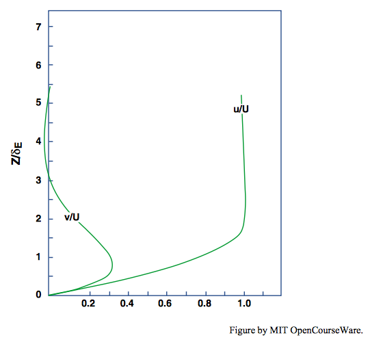
The thickness of the bottom Ekman layer should depend on the viscosity of the fluid and on the Coriolis parameter. These two factors work against one another: the greater the viscosity, the greater the thickness affected by friction, and the greater the Coriolis effect, as measured by the Coriolis parameter \(f\), the less the thickness. The conventional measure of the Ekman-layer thickness is \([A_{V}(f / 2)]^{1 / 2}\), conventionally denoted by \(\delta_{E}\). (Do not be concerned with the reasons for the factor \(2\) in the denominator.) Upward in the Ekman layer the effect of friction tails off rapidly, but keep in mind that the upper limit is indefinite: the velocity decreases upward as a negative exponential function of height above the bottom boundary. It is best to view \(\delta_{E}\) as representative of the thickness of the Ekman layer; in the parlance of geophysical fluid dynamics, the Ekman-layer thickness is of order \(\delta_{E}\). Finally, it will probably seem counterintuitive to you that the thickness of the Ekman layer does not depend on the geostrophic velocity.

As is so often the case, the value to use for the kinematic viscosity in the theory for the bottom Ekman layer is a problem. The molecular kinematic viscosity \(\nu\) could be used, and that gives an exact solution for a laminar Ekman layer. The problem is that the mean-flow Reynolds numbers of large-scale flow in both the ocean and the atmosphere are so large that the Ekman layer must be turbulent rather than laminar. Alternatively, the eddy viscosity \(A_{V}\) can be used, but you have seen earlier that the eddy viscosity is itself a function of the flow, rather than a property of the fluid, and it might be expected to vary with height above the bottom boundary. With what seem to be reasonable values of eddy viscosity, the Ekman-layer thickness is on the order of some tens of meters, which is about what has been observed in the atmosphere and oceans.