
6.4: Wave Boundary Layers
- Page ID
- 4186

The linearized small-amplitude solution for velocity mentioned in the previous section predicts spatially slowly varying velocities both at and below the water surface at any given time. In the case of waves in shallow to intermediate water depths (that is, for which the wavelength is not very small relative to the water depth), these velocities are predicted to be still appreciable even at the bottom—and when the wavelength is large relative to the water depth, the magnitudes of near-bottom velocities are about the same as the velocities at the surface. Remember that the assumption of inviscid flow means that these nonzero near-bottom velocities extend all the way to the bottom.
Viscosities of real fluids like water are small enough that the free- surface profile and the spatial and temporal distribution of velocities is well accounted for by the inviscid solutions, and viscous damping is small—so small that large waves can travel across wide ocean basins without great loss of energy. But the predicted nonzero velocities at the solid bottom boundary under the waves is clearly contrary to fact: just as in unidirectional flows of real fluids, the velocity must go to zero at the bottom boundary. This leads to the concept of the bottom boundary layer in oscillatory flows: this is commonly called the wave boundary layer.
Many of the physical effects associated with wave boundary layers are analogous to or parallel to those of unidirectional-flow boundary layers. Here is a mostly qualitative account of some of the important things about wave boundary layers. The first thing to note is that, just as with unidirectional flows, at relatively low values of a suitably defined Reynolds number the boundary layer is laminar, and at higher values of the Reynolds number the boundary layer is turbulent, even though the flow in the domain above the boundary layer, where the inviscid assumption holds, is effectively nonturbulent (provided that there is no coexisting unidirectional current; see a later section).
If the wave Reynolds number is defined as \(\rho U_{m} d_{\text{o}} / \mu\), where \(U_{m}\) is the maximum bottom velocity predicted by the inviscid theory and \(d_{\text{o}}\) is orbital diameter given by the inviscid theory, then the critical value for the transition from laminar to turbulent flow in the wave boundary layer is known from observations in wave tanks and oscillatory flow ducts in the laboratory to be about \(10^{4}\).
An exact solution can be found for the velocity profile in the laminar boundary layer. The mathematics is straightforward but beyond the scope of these notes. The result, when expressed as the velocity deficit \(u_{d}\), the difference between the inviscid bottom velocity (which in the context of the laminar boundary can be viewed as the velocity at the top of the boundary layer) and the actual velocity at some height \(z\) above the bottom, is
\[u_{d}=e^ {\left(-\sqrt{\frac{\omega}{2 v}} z\right)} \cos \left(k x-\omega t+\sqrt{\frac{\omega}{2 v}} z\right) \label{6.1} \]
where \(\omega\) is the angular frequency of the oscillation (related to the period \(T\) by \(\omega = 2\pi /T\)), \(k\) is the wave number (related to the wavelength \(L\) by \(k = 2\pi /L\)), \(ν\) is the kinematic viscosity \(\mu /\rho\), and \(z\) is measured upward from the bottom.
The solution in Equation \ref{6.1} has two factors, one expressing a negative exponential dependence and the other expressing a cosine dependence. The former causes \(u_{d}\) to drop off sharply with height above the bottom, and the latter just takes account of the time variation in the velocity—but it is important to note that there is a phase difference with the overlying inviscid flow, and the phase difference itself depends on \(z\), ranging upward from zero at the bottom at the same time \(u_{d}\) is getting smaller.
The negative exponential dependence of \(u_{d}\) on \(z\) in Equation \ref{6.1} means that the effective boundary-layer thickness is fairly well defined, although technically one has to take some arbitrary value like \(0.01\) for \(u_{d}\) in order to obtain a definite thickness for the boundary layer. It turns out that the value of \(z\) that corresponds to \(u_{d} = 0.01\), which is usually denoted by \(\delta_{L}\), is
\[z=\delta_{L}=5 \sqrt{\frac{2 v}{\omega}} \label{6.2} \]
But most boundary layers under waves in the real ocean under conditions of interest in sediment transport are turbulent rather than laminar. Theoretical analyses of the turbulent wave boundary layer have been carried out by replacing the molecular viscosity by a turbulent eddy viscosity, making some assumption about how the eddy viscosity varies vertically, and obtaining an expression for the vertical velocity distribution. The velocity profile is found in this way to be logarithmic. Again there is the problem of how to define arbitrarily the boundary-layer thickness, but the height \(\delta_{T}\) of the turbulent boundary layer is usually taken to be
\[\delta_{T}=\frac{2 \kappa u_{*}}{\omega} \label{6.3} \]
where \(\kappa\) is von Kármán’s constant, the inverse of the constant \(A\) introduced in Chapter 4, and \(u_{*}\) is again the shear velocity (which could be taken as the maximum or the time average).
A significant aspect of wave boundary layers is that they do not keep growing upward into the interior of the flow indefinitely, the way unidirectional- flow boundary layers do, provided that density stratification does not inhibit their upward growth. The reason is that the thickness of the wave boundary layer is limited by the cessation and turnaround of the flow in each cycle. For turbulent wave boundary layers over rough beds, the thickness of the wave boundary layer is likely to be something less than one meter—far smaller than the typical boundary layer beneath currents in deep-water natural environments.
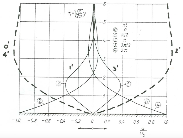
Just to give you a feel for the velocity structure in the oscillatory-flow boundary layer is like, Figure \(\PageIndex{1}\) is a graph (admittedly somewhat complicated) that shows flow velocity in the laminar oscillatory boundary layer vs. height above the bottom for four equally spaced times during one complete oscillation cycle (\(0\), \(\pi /2\), \(\pi\), \(3\pi /2\), and \(2\pi\)). The vertical coordinate is labeled with values of the length variable under the radical sign in Equation \ref{6.2} but with slightly different notation. The curves in Figure \(\PageIndex{1}\) are labeled in two ways: \(1–4\) unprimed, and \(1–4\) primed. The unprimed numbers are for what the velocity of the bottom would look like to a neutrally buoyant observer riding with the oscillatory flow just outside the boundary layer. This corresponds to oscillating a flat plate in a tank of still water. The primed numbers are for the equivalent curves, more relevant to our interests here, that show the velocity profile of the fluid relative to an observer planted firmly on the bottom. You can see how, during each half cycle (for example, from curve \(0^{\prime}\) to curve \(1^{\prime}\) to curve \(2^{\prime}\)) there is a considerable mismatch in phase between the upper part of the boundary layer and the lower part.
Finally, the magnitude of the bottom shear stress is important both for its role in sediment transport and also for its effect on attenuation of wave energy by bottom friction, so a lot of effort has gone into developing ways to predict the bottom shear stress. Basically it boils down to dealing with a wave friction factor \(f_{w}\), analogous to the unidirectional-flow friction factor, and working with an experimentally determined wave friction-factor diagram expressing the dependence of the wave friction factor on the Reynolds number and, for rough beds, a relative roughness \(d_{\text{o}}/D\), where \(D\) is the size of the roughness elements.
One interesting aspect of the bed shear stress in oscillatory flow is that in laminar boundary layers the maximum shear stress leads the maximum velocity by a phase angle of \(\pi /4\), meaning that the maximum shear stress acts on the bottom at a time equal to \(T/8\) (where \(T\) is the period of the oscillation) before the velocity reaches its maximum at the top of the boundary layer. In turbulent boundary layers the same effect is present but the phase difference is somewhat smaller.