
5.6: Hydraulic Regimes of Open-Channel Flow
- Page ID
- 4181

Now that you know about supercritical vs. subcritical flow as well as about laminar vs. turbulent flow, various phenomena of open-channel flow can be drawn together into a single graph, to give you an idea of the wide range of hydraulic regimes of flow that can exist. Figure \(\PageIndex{1}\) is a graph of mean flow depth against mean flow velocity for steady uniform open-channel flow in a wide rectangular channel. If bed roughness is present, its height is assumed to be a small fraction of the flow depth. Both depth and velocity span several orders of magnitude, a far greater range than is found in the sediment-transporting flows encountered in natural flow environments.
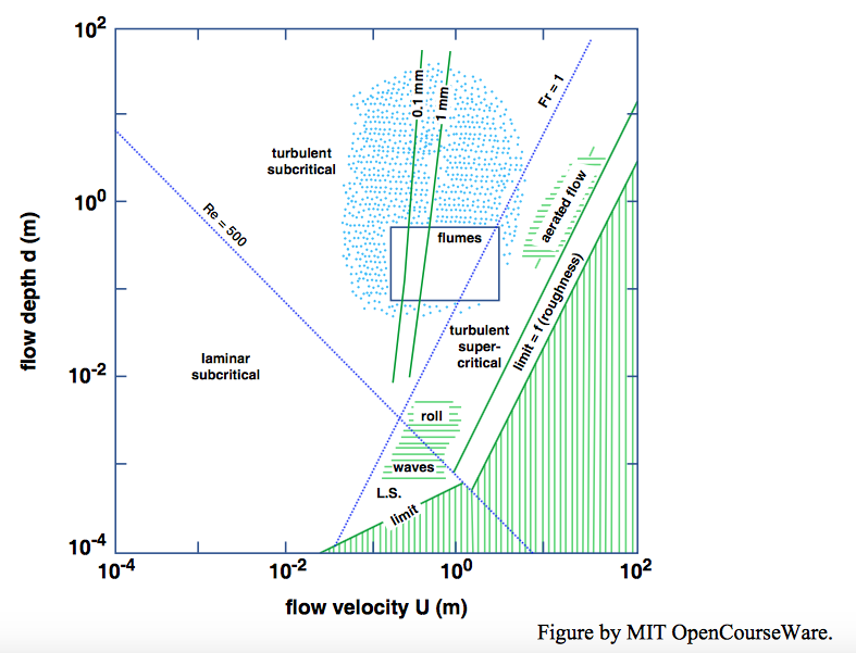
It is easy to plot curves in Figure \(\PageIndex{1}\) corresponding to \(\text{Fr} = 1\), for the transition between subcritical flow and supercritical flow, and to \(\text{Re} = 500\) (\(\text{Re}\) based on flow depth), for the transition between laminar flow and turbulent flow. In a \(log–log\) plot like Figure \(\PageIndex{1}\) both of these conditions plot as straight lines; the line for \(\text{Fr} = 1\) slopes upward to the right, and the line for \(\text{Re} = 500\) slopes downward to the right. These two lines partition the graph into four sectors: turbulent subcritical in the upper left (the most common in natural open-channel flows), turbulent supercritical in the upper right, laminar subcritical in the lower left, and laminar supercritical in the lower right.
The usefulness of a graph like Figure \(\PageIndex{1}\) is that it helps to put into perspective the wide range of open-channel flows. The flow regimes shown in Figure 5.5.3 are just extensions of the concept of flow regimes introduced in the discussion of flow around a sphere in Chapter 3.
In the lower part of Figure \(\PageIndex{1}\) are two curves (one for laminar flow and the other for turbulent flow) sloping upward to the right, below which steady, uniform open-channel flows cannot exist. These curves are defined by the condition that channel slope approaches the vertical, giving the greatest gravitational driving force possible. It is easy to get an exact solution for the curve that expresses this condition for laminar flow, by integrating Equation 4.7.6 to find the mean velocity \(U\) as a function of flow depth, fluid properties \(\gamma\) and \(\mu\), and channel slope angle \(\phi\), and then taking \(\sin \phi=1\), giving \(U=d^{2} \gamma / 3 \mu\). This plots as a straight line in \(\PageIndex{1}\). A sheet of rainwater running down a soapy windowpane is an example of flows represented by this line.
It is not as easy to obtain the limiting curve for turbulent flows, because we have to work with a resistance diagram like that in Figure 4.7.11. The curve shown in Figure \(\PageIndex{1}\) was drawn in an approximate way by obtaining the friction factor \(f\) from the smooth-flow curve in Figure 4.7.7 and using that value together with \(\tau_{0}=\gamma d \sin \alpha\) in Equation 4.6.4. Figure 4.7.7 is for circular pipes, but it should be roughly applicable to open-channel flow provided that the pipe diameter is appropriately replaced. Four times the flow depth was used in place of pipe diameter in computing the Reynolds number in Figure 4.7.7, because as noted in Chapter 4 the hydraulic radius of a circular pipe is one-fourth the pipe diameter, whereas the hydraulic radius of a very wide open-channel flow is just about equal to the flow depth. For rough flows the limiting curve in Figure 5.5.3 would be displaced upward somewhat, because the friction factor is greater for a given Reynolds number.