
4.8: More on the Structure of Turbulent Boundary Layers- Coherent Structures in Turbulent Shear Flow
- Page ID
- 4859

There was a time, until the 1960s, when the emphasis in turbulence research was statistical: turbulence was largely viewed as a strictly random phenomenon, one that can be analyzed only by statistical methods. Implicit in such an approach is that turbulence has no apparent regularity or “ordered-ness” in its structure.
Beginning in the 1960s, however, there have been many studies on what are now termed coherent structures in turbulent shear flow. (I postponed this material until now, so that you would have more background in turbulent shear flow to bring to it.) It has become clear that shear turbulence is not merely a random assemblage of eddies of all sizes, shapes, and magnitudes and orientations of vorticity; rather, these are irregular but repetitive eddy structures, or flow patterns, in time and space, with distinctive shapes and histories of formation, evolution, and dissipation. These coherent structures are not strictly regular in geometry or periodic in time, but nonetheless they have a strong and distinctive element of non- randomness. One way of describing these coherent structures is that they are quasi-regular, or quasi-periodic, or quasi-deterministic. (The word quasi in Latin means “almost”.) Admittedly the foregoing characterization does not give you much basis for imagining or visualizing what the coherent structures look like; see below for more concrete material.
Recall from Chapter 3 that turbulence can be viewed as an assemblage of swirling and intergrading parcels of fluid, called eddies, on a wide range of scales. Eddies have vorticity: the fluid in the eddies undergoes rotational motion, which is described by the local rate and orientation of rotation, varying from continuously from point to point. To appreciate the nature of coherent structures in shear turbulence, you need to deal with the shapes and also the vorticity of the structures, and how the shape and the vorticity develop ands change during the lifetime of a given element of structure.
The best way to perceive or capture ordered structures is to visualize them, by supplying the flow with marker material that reveals or distinguishes differently moving regions of fluid. Studies of ordered structures in turbulent flow have mostly used three techniques flow visualization:
- dye injection, at points or along lines
- generation of lines of tiny hydrogen bubbles in water by passing a current through a fine platinum wire immersed in the flow
- high-speed motion-picture photography of very small opaque solid particles suspended in the flow
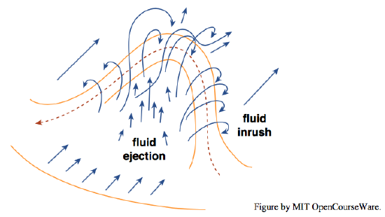
It is generally agreed that flow near the boundary in a turbulent shear flow tends to be characterized by the following sequence of events, commonly called the burst–sweep cycle. A high-velocity eddy or vortex (called a sweep) moves toward the boundary and interacts with low velocity fluid near the boundary to cause acceleration, increase in shear, and development of small-scale turbulence; this accelerated fluid is then lifted from the boundary and ejected as a turbulent burst into a region of flow farther from the boundary. The sweeps are inrushes of high-seed fluid at at a shallow angle toward the wall; the bursts are violent ejections of low- speed fluid outward from the vicinity of the wall.
Close to the boundary the high-velocity and low-velocity vortices or eddies tend to be elongated or streaked out in the streamwise direction, and their manifestation is a streaky or ribbon-like pattern of high and low fluid velocities, and therefore of boundary shear stresses as well. Owing to the substantial changes in velocity, shear, and turbulence above a given point on the boundary occasioned by the bursting cycle, the effective thickness of the viscous sublayer varies with time. Because of the existence of the burst–sweep cycle, the picture of the viscous sublayer developed earlier in this chapter is oversimplified: it has a definite thickness only as a time average at a given point. At a given time, the viscosity-dominated layer near the bottom is in some regions thin (and in those regions, shear near the bed, and shear stress on the bed, are temporarily high), and in adjacent regions it is thicker (and in those regions, the shear and the bed shear stress are temporarily smaller).
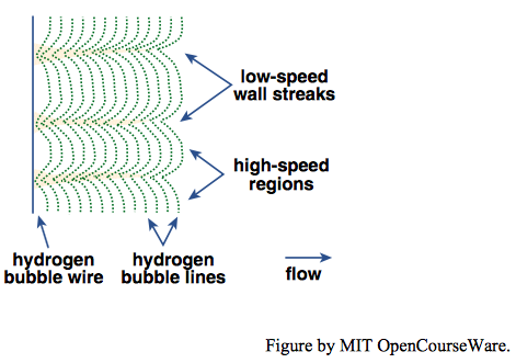
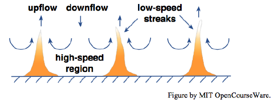
The common visual manifestation of the burst–sweep cycle is the existence of streamwise-oriented low-speed streaks (also called wall-layer streaks, or just streaks) just above the flow boundary. These streaks are low-speed zones that lie between intervening high-speed zones. In the low- speed zones, slow-moving fluid has an upward (that is, in the direction away from the boundary) component of motion as a result of downward flow in the high-speed zones (Figures \(\PageIndex{1}\), \(\PageIndex{2}\)). Sediment particles tend to be swept into the low-speed streaks as the faster-moving fluid in the high-speed zones moves slightly obliquely toward the low-speed zones.
You might have seen such low-speed streaks on a cold winter day, with temperatures well below freezing, when a wind-driven light snow first falls upon are pavement, or in the desert when a strong wind blows fine sediments across the road surface. It is not difficult to set up a beautiful visual demonstration of low-speed streaks in a laboratory flume, where a small concentrations of brilliant white sediment particles are transported across a dark-colored bare flume bottom.
The strong message from such visualizations is that
- the streaks are strongly elongated parallel to the flow direction;
- the streaks waver and shift irregularly from side to side; and
- the streaks appear and disappear with time.
Much effort has gone into study of the scale of the streaks. It is clear that for dynamically smooth flow the average spacing \(\lambda\) of the streaks, when nondimensionalized as \(\lambda^{+}=\rho \lambda u_{*} / \mu\), is in the range somewhat above or below \(100\), and only weakly dependent upon the mean- flow Reynolds number. The streaks are also present when the flow is dynamically fully rough; the spacing of the streaks, when nondimensionalized by dividing by the size of the close-packed roughness elements, is between \(3\) and \(4\). In transitionally rough flow, the situation is less straightforward.
The burst–sweep cycle and its associated streak structure is a feature of the near-boundary part of the inner layer, in what was called in an earlier section the viscous sublayer (if one is present) and the buffer layer. Farther away from the boundary, where eddy scales range to larger size and where both production and dissipation of turbulent kinetic energy are less, there seems to be less coherence in the structure of the turbulence.
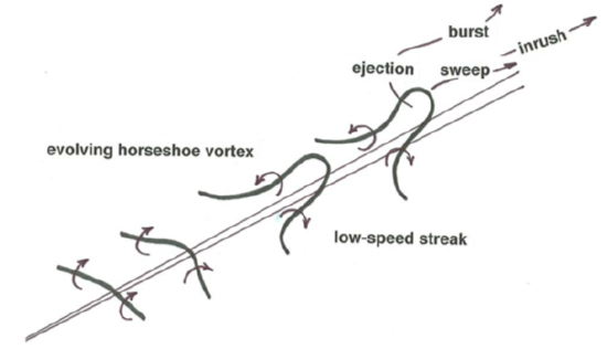
It remains to look into how the counter-rotating vortices, stretched out in the streamwise direction, originate, and how their shapes evolve. It is generally accepted that the key features in this regard are vortices variously called horseshoe vortices or hairpin vortices, owing to their characteristic shape (Figures \(\PageIndex{3}\), \(\PageIndex{4}\)). These vortices develop, in ways not yet well understood, and then become stretched downstream by the strong mean shear, and as they are stretched, the vorticity in the limbs increases. (In an approximate sense, as the diameter of the spinning fluid is decreased, the spinning is compressed into a smaller cross section, and the rate of spinning increases.) These elongated vortex limbs are generally believed to be responsible for the fluid motions in the burst–sweep cycle.
The study of coherent structures in turbulent shear flows is an active area of research. For informative reviews of the status of understanding, see Robinson (1991), Grass and Mansouri-Tehrani (1996), and Smith (1996). Also on the reading list at the end of the chapter are some of the classic papers: Kline et al. (1967), Corino and Brodkey (1969), Grass (1971), and Offen and Kline (1974, 1975).
Chapter 4 References Cited
Coleman, N.L., 1981, Velocity profiles with suspended sediment: Journal of Hydraulic Research, v. 19, p. 211-229.
Corino, E.R., and Brodkey, R.S., 1969, A visual investigation of the wall region in turbulent flow: Journal of Fluid Mechanics, v. 37, p. 1-30.
Grass, A,J,, and Mansour-Tehrani, M, 1996, Generalized scaling of coherent bursting structures in the near-wall region of turbulent flow over smooth and rough boundaries, in Ashworth, P.J., Bennett, S.J., Best, J.L., and McLelland, S.J., Coherent Flow Structures in Open Channels: Wiley, p. 41-61
Grass, A.J., 1971, Structural features of turbulent flow over smooth and rough boundaries: Journal of Fluid Mechanics, v. 50, p. 233-255.
Grass, A.J., Stuart, R.J., and Mansour-Tehrani, M, 1991, Vortical structures and coherent motion in turbulent flow over smooth and rough boundaries: Royal Society (London), Philosophical Transactions, v. A336, p. 35-65.
Hinze, J.O., 1975, Turbulence, Second Edition: McGraw-Hill, 790 p.
Izakson, A., 1937, Formula for the velocity distribution near a wall [in Russian]: Zhurnal’ Eksperimental’noi i Teoreticheskoi Fiziki, v. 7, p. 919-924.
Kline, S,J., Reynolds, W.C., Schraub, F.A., and Runstadler, P.W., 1967, The structure of turbulent boundary layers: Journal of Fluid Mechanics, v. 95, p. 741-773.
Millikan, C.B., 1939, A critical discussion of turbulent flow in channels and circular tubes: Fifth International Congress on Applied Mechanics, Cambridge, Massachusetts, Proceedings, p. 386-392.
Monin, A.S., and Yaglom, A.M., 1971, Statistical Fluid Mechanics, Volume 1: Cambridge, Massachusetts, MIT Press, 769 p.
Morris, H.M., 1955, Flow in rough conduits: American Society of Civil Engineers, Transactions, v. 120, p. 373-398.
Nikuradse, J., 1933, Gesetzmässigkeiten der Turbulente Strömung in glatten Rohren: VDI Forschungsheft 356.
Offen, G.R., and Kline, S.J., 1974, Combined dye-streak and hydrogen- bubble visual observations of a turbulent boundary layer: Journal of Fluid Mechanics, v. 62, p. 223-239.
Offen, G.R., and Kline, S.J., 1975, A proposed model of the bursting process in turbulent boundary layers: Journal of Fluid Mechanics, v. 70, p. 209-228.
Robinson, S.K., 1991, Coherent motions in the turbulent boundary layer: Annual Review of Fluid Mechanics, v. 23, p. 601-639.
Smith, C.R., 1996, Coherent flow structures in smooth-wall turbulent boundary layers: facts, mechanisms and speculation, in Ashworth, P.J., Bennett, S.J., Best, J.L., and McLelland, S.J., Coherent Flow Structures in Open Channels: Wiley, p. 1-39.
Tennekes, H., and Lumley, J.L., A First Course in Turbulence: Cambridge, Massachusetts, MIT Press, 300 p.
Theodorsen, T., 1952, Mechanisms of Turbulence: 2nd Midwestern Conference on Fluid Mechanics, Ohio Sate University, Columbus, Ohio, Proceedings, p. 1-18.
Tritton, D.J., Physical Fluid Dynamics, Second Edition: Oxford University Press, 519 p.