9.4: Movement Threshold
- Page ID
- 4207

How is the Threshold for Movement Identified?
At this point, as a prelude to looking at the various diagrams that are in common use for incipient movement, it seems appropriate to pose the following fundamental question: How is the condition of incipient movement identified? An untutored outside observer might naturally assume that the answer is to watch the sediment bed to determine when, under conditions of slowly increasing flow strength, the sediment begins to move. But there is a serious problem with such a procedure, as can easily be demonstrated by a simple flume experiment: even for bed shear stresses (or flow velocities) that are well below what would conventionally be considered to represent the threshold or critical condition for sediment movement, some bed particles are moved by the flow. It is easy to understand why this is so. Recall from the material on turbulence in Chapter 3 that because of the impingement of turbulent eddies on the sediment bed the instantaneous fluid forces on sediment particles varies widely. The consequence is that even in weak flows a particularly strong turbulent eddy would occasionally cause one or more particles to move. There is thus a wide range of flow conditions that cause weak sediment movement. Put another way, the question becomes: How long should one wait to detect movement of a particle on the sediment bed? A minute? An hour? A day?
The wide range of bed shear stresses for which there is weak particle motion brings forth an additional question: Does a threshold bed shear stresses for incipient movement really exist? Some would contend that the range of bed shear stresses for weak particle motion is indefinitely wide, and that because of that there is a conceptual flaw in the assumption that a definite threshold condition can be defined. It is true that the weaker the flow, the smaller the number of bed particles that are moved by the flow (per unit time and per unit area of the bed), but the lower limit for any particle motion is indefinite. For a cogent exposition of the impossibility of assigning a definite threshold condition, see the paper by Lavelle and Mofjeld (1987).
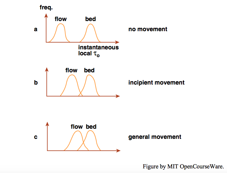
This difficulty in defining the condition of incipient movement is largely because incipient movement is stochastic, in that the instantaneous resultant force on a bed particle varies irregularly through time just as does, say, a turbulent velocity component. One conceptually satisfying way of looking at the threshold of sediment movement is in terms of the relationship between two different probability frequency distributions: the distribution of instantaneous local \(\tau_{\text{o}}\) needed to move the set of particles occupying some area of the bed surface, and the distribution of instantaneous local τo that acts on any small area of the bed, of about the size of the particles, through time (Figure \(\PageIndex{1}\); after Grass 1970). When the two distributions do not overlap (Figure \(\PageIndex{1}\)A), the flow is never strong enough to move any of the particles on the bed, whereas when the two distributions overlap somewhat (Figure \(\PageIndex{1}\)B), there is a subset of particles on the bed surface which can be, and therefore are, moved by the flow. With increasing flow strength the distributions come to overlap entirely (Figure \(\PageIndex{1}\)C), meaning that all the particles on the bed surface are susceptible to movement. When the condition for movement threshold is viewed in this way, it is easy to identify the basis for the skeptics’ view that it is not possible to define the condition of incipient movement: they would argue that the right-hand (high flow strength) tail of the frequency distribution of instantaneous local \(\tau_{\text{o}}\) extends indefinitely far to the right, toward higher bed shear stresses. One could argue, of course, that if the time average of the instantaneous shear stress is sufficiently small, none of the bed particles would ever move, but that condition is so far from the conventional view of the movement threshold as to be irrelevant to the problem, in a practical sense.
Here we take the approach, in common with most sedimentationists, that the concept of a threshold for sediment movement has a certain physical reality, despite the uncertainty described above, and that techniques must be available to identify the threshold condition. There are two ways to attempt to identify the threshold condition, which might be termed, unofficially, the watch- the-bed technique and the reference-transport-rate method.
The watch-the-bed method: as mentioned at the beginning of this section, this is in a sense the most natural way of defining the threshold condition. The problem of the wide range of conditions of weak sediment movement might be circumvented by general agreement, by convention, about where in this range of weak movement the threshold condition is situated. As you can imagine, much of the scatter in data on movement threshold is the result of differing views in this respect.
There have been attempts at quantifying the conditions for incipient movement. Neill (1968) and Yalin (1977) argued that kinematic similarity of movement of grains implies identity of the dimensionless parameter \(N=n D^{3} / u_{*}\), where \(n\) is the number of grains in motion per unit area and unit time. They suggested adopting \(10^{-6}\) as a practical critical value of \(N\), and pointed out that, for equal values of the Shields parameter must be \(30\) times greater in air than in water, so that for equal \(N\), \(n\) must be \(30\) times greater. Such attempts at quantification have never come into general use.
The reference-transport-rate method: A second way of defining the threshold condition is to circumvent the uncertainty about when movement begins by defining some small value of the dimensionless unit sediment transport rate that seems to correspond most closely to what the consensus view of the threshold condition is, and assume, for practical purposes, that that value represents the threshold condition. There will be more on the reference-transport-rate method in the later chapter on mixed-size sediments.
In practice, what has to be done is to make a fairly large number of measurements of the dimensionless unit sediment transport rate at a number of flow strengths above the threshold, plot the results, fit a curve to the results in some way, either as an analytical function of just “by eye”, and then extrapolate (or interpolate, if at least one of the data points lies below the reference condition) to find the value of bed shear stress associated with the reference transport rate.
There is a potential inconsistency between the two methods described in the preceding paragraphs. In the watch-the-bed method, a flume run is usually set up with an initially planar bed, and the bed is watched for signs of particle movement on that planar bed. In the reference-transport method, the measurements are usually made after the sediment transport has come into equilibrium with the flow, and there is the possibility that bed forms, especially ripples, have formed on the bed. The sediment transport rate over a rippled bed is in general different from that over a planar bed of the same sediment experiencing the same flow conditions—so the threshold condition is identified in a fundamentally different situation.
Representations of the Movement Threshold
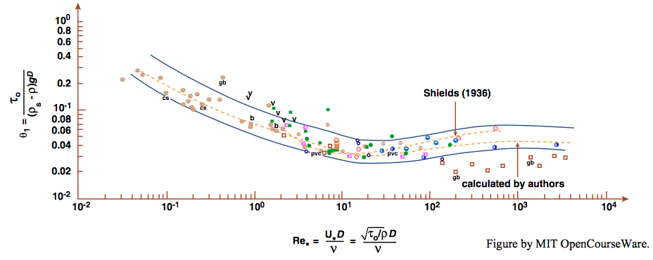
What has traditionally been done, in studies of incipient movement, is to plot experimental results in a graph with the axis variables arranged in such a way that a unique curve in the graph separates conditions of established movement from conditions of no movement. The earliest such work is that of Shields (1936), who plotted initial-movement data from flume experiments on a graph of boundary shear stress nondimensionalized by dividing by the submerged specific weight and the mean size of the sediment (the resulting dimensionless variable is now called the Shields parameter; see the section on variables in Chapter 8) against the boundary Reynolds number. The result was not the first such attempt, but it became firmly established, especially in the field of hydraulic engineering, by virtue of its rational basis in fluid dynamics.
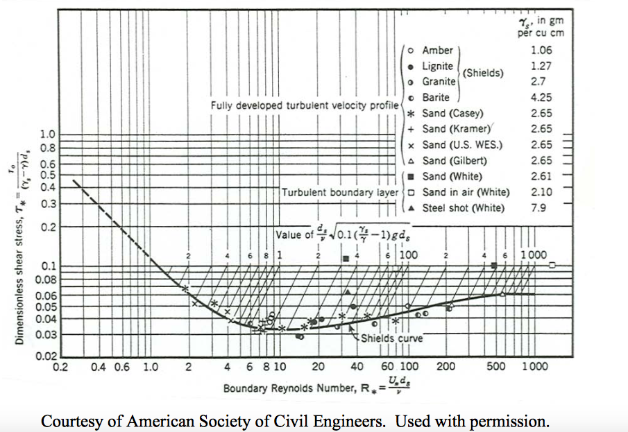
The experimental results obtained by Shields himself, together with some earlier data. The threshold is called the Shields curve. There are two striking things about Figure \(\PageIndex{2}\):
- There is considerable scatter in the points.
- Shields had no data for \(\text{Re}_{*}\) less than about \(2\) or greater than \(600\).
It helps to evaluate the significance of the Shields diagram if you understand more clearly how the data were obtained. Shields made his experiments in flumes \(0.8\) \(\mathrm{m}\) and \(0.4\) \(\mathrm{m}\) wide, with beds composed of granite fragments \(0.85\) \(\mathrm{mm}\) to \(2.4\) \(\mathrm{mm}\) in diameter, coal (\(\rho_{s} = 1.27\) \(\mathrm{g/cm^{3}}\)) \(1.8\) \(\mathrm{mm}\) to \(2.5\) \(\mathrm{mm}\) in diameter, amber (\(\rho_{s} = 1.06\) \(\mathrm{g/cm^{3}}\)) \(1.6\) \(\mathrm{mm}\) in diameter, and barite (\(\rho_{s} = 4.2\) \(\mathrm{g/cm^{3}}\)) \(0.36\) \(\mathrm{mm}\) to \(3.4\) \(\mathrm{mm}\) in diameter. Bed shear stress was determined from the resistance equation, \(\tau_{\text{o}}=\gamma d \sin \phi\) (Chapter 4 in PartI). The bed was carefully leveled before each run. Discharge and therefore mean velocity were increased in steps, and the slope was adjusted to maintain uniform flow. After grains began to move on the bed, bed load was collected in a trap at the end of the flume so that the rate of sediment transport for a given condition could be determined. For each bed material several observations were made at different discharges and rates of sediment transport, and the beginning of grain movement was determined not so much by direct observation as by plotting the measured rates of transport and extrapolating to the value of \(\tau_{\text{o}}\) that corresponded to zero rate of transport. (Shields did not report exactly how he made the extrapolation.) Shields observed that this corresponded to what other workers had described as “weak movement” of particles.
Shields himself noted that small ripples tend to form on the bed as soon as particles start to move. The presence of these ripples affects the rate of bed-load movement, so there is some question about exactly what was being determined when Shields extrapolated the measured rates to zero: initiation of movement on a plane bed, or initiation of movement on a rippled bed?
It has been observed by other workers that the critical shear stress for initiation of particle movement on a rippled bed is greater than for that on a plane bed, although the mean velocity of flow is less. The explanation is that ripples create form resistance, which contributes most of the measured average bottom shear stress. If the depth does not change, the slope of the flume has to be increased to produce the shear stress needed to balance this form resistance and produce the same velocity. It is observed, however, that the slope and velocity needed to move particles on a rippled bed can be reduced below that necessary to move particles on a plane bed, because the phenomenon of flow separation over the ripples produces locally high and widely fluctuating shear stresses on the bed, which are large enough to move grains even at mean flow velocities lower than those required to move grains on a plane bed.
To make this more explicit, imagine setting up two series of flume experiments, side by side, with exactly the same flow depth and flow velocity, one with a planar sediment bed and one with a rippled bed. Start at a velocity so low that there is no particle movement in either flume. Because of the large form drag on the rippled bed, slope and therefore boundary shear stress is much greater than for the planar bed. Now gradually increase flow velocity in both flumes while keeping flow depth constant but increasing the slope to maintain uniform flow. Boundary shear stress thus increases in both flumes, but at all times it is greater on the rippled bed than on the planar bed. Particle movement starts first on the rippled bed; eventually, at a substantially higher flow velocity, particles begin to be moved on the planar bed also, but boundary shear stress on the planar bed at that point turns out to be lower than that for which particle movement began on the rippled bed.
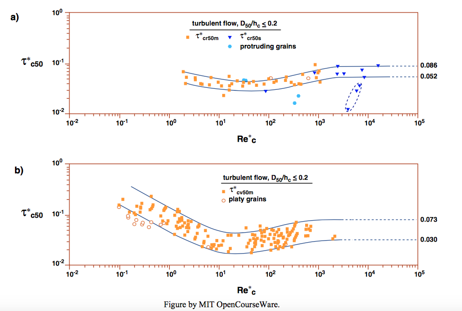
The original Shields diagram has been used with little modification right up to the present, especially by hydraulic engineers. Miller et al. (1977) updated the Shields diagram, by drawing upon various more recent data to replot the diagram and redraw the curve; see Figure \(\PageIndex{3}\). The Miller et al. diagram is also in wide use. More recently, Buffington and Montgomery (1997) made an exhaustive and systematic compilation and analysis of studies on movement threshold. They were able to identify a systematic difference in the position of the Shields curve in the Shields diagram between data obtained by the watch-the- bed method and the reference-transport-rate method (Figure \(\PageIndex{4}\)). They found a systematic difference in the location of the Shields curve, such that the curve based on the reference-transport-rate method lies above the curve based on the watch-the-bed method.