7.3: The Rossby Number and Inertia Currents
- Page ID
- 4192

The Rossby Number
How can we gain a general idea about whether the motion of a fluid or a solid object on or near the Earth’s surface would manifest non-negligibly the Coriolis effect? The answer lies in a dimensionless parameter called the Rossby number. Any such motion, whether it is a flow of a fluid or the flight of a bullet or an artillery shell or a rocket, has some characteristic speed \(U\) and moves over some characteristic distance \(L\). Depending upon the latitude, there is some particular value of the Coriolis parameter, ranging from zero at the Equator to a maximum at the poles. The essential idea is this: how long does it take for the material to make its trip, in comparison to how much the Earth rotates under the material while it is making its trip?
The only way to combine the three variables \(U\) with dimensions of length/time), \(L\) (with dimensions of length), and \(f\) (with dimensions of \(1\)/length) is \(U/fL\), which is one form of what is called the Rossby number. You can think of the Rossby number as the ratio of two velocities, because the combination \(fL\) has the dimensions of a velocity. In the case of the ocean current, moving at a few centimeters per second over a distance of, say, a thousand kilometers, the Rossby number is very small; in the case of a speeding bullet, the velocity is very large and the distance of travel is no more than something like a thousand meters, the Rossby number is very large. In other words, the Earth rotates quite a lot in the time it takes for the ocean current to move from place to place, so the effect of the Earth’s rotation on the movement of the fluid is great. By contrast, the Earth rotates very little in the time it takes the bullet to travel from the rifle to the target, so the Coriolis acceleration is negligible.
Inertia Currents
I mentioned earlier that you might generate a current in the interior of the big pan on your turntable and then study the effect of the Coriolis acceleration on that current. If the pan is broad enough and deep enough, the mass of water you set in motion can move for quite some time and distance just by its own inertia before being brought to a stop by friction forces exerted by the adjacent fluid. Currents of this kind are called inertia currents. In nature they might be produced by passage of a sudden squall or a fast-moving windstorm over a large body of water.
Consider a small parcel of water anywhere in your inertia current. Your first thought might be that, because no forces are acting on it, it would move in a straight line at constant speed—and that would be true, if your turntable were not rotating. But remember that, from the standpoint of an observer on the turntable, the rotation of the turntable results in a Coriolis acceleration, so you have to deal with a force per unit mass of fluid equal to \(fv\), the Coriolis acceleration (\(v\) is the velocity and \(f\) is the Coriolis parameter), acting at right angles to the direction of movement. If the turntable is rotating counterclockwise as viewed from above, then the Coriolis force acts to the right of the direction of movement. That sense of rotation is the same as in the Northern Hemisphere on the Earth. If the turntable is rotating clockwise, then the Coriolis force acts to the left of the direction of movement, as in the Southern Hemisphere.
The dynamicist’s approach to the problem of how the water in the inertia current moves as a function of time is to derive the governing equations of motion, including pressure forces, viscous forces, gravity forces, and Coriolis forces, and then specialize the equations for the particular flow, making any judicious simplifications necessary for good mathematical progress. We will not go through such an exercise here. For inertia currents the equations simplify very nicely, just because we are assuming that the only force we have to deal with is the Coriolis force.
When written in an \(xyz\) coordinate system with reference to the horizontal plane at some point on the Earth (\(z\) being vertical, \(x\) being east, and \(y\) being north), the two horizontal equations come out to be just
\begin{array}{l}{\frac{d u}{d t}=2 v \omega \sin \phi} \\ {\frac{d v}{d t}=-2 u \omega \sin \phi} \label{7.3} \end{array}
or, using the notation for the Coriolis parameter,
\begin{array}{l}{\frac{d u}{d t}=f v} \\ {\frac{d v}{d t}=-f u} \label{7.4} \end{array}
where \(u\) and \(v\) are the \(x\) and \(y\) components, respectively, of velocity of the fluid relative to the horizontal plane defined above.
Do not worry about the signs in front of the Coriolis terms; they come about when the \(x\) and \(y\) components of the Coriolis acceleration are derived for the horizontal plane. This is a simple set of equations. Its solution, for an initial condition that \(u = U\) and \(v = 0\) at \(t = 0\), is
\begin{array}{l}{u=U \cos ft} \\ {v=-U \sin f t} \label{7.5} \end{array}
If you go back to your storehouse of mathematical knowledge you can easily demonstrate to yourself that this solution represents motion around a circle at constant speed, with the time \(t\) as a parameter. For circular motion like this, the radius of the circle is just \(U/f\), and the time it takes a particle to go all the way around the circle is \(2 \pi /f\). This circle is called an inertia circle, and the period is called the inertia period.
That the water in an inertia current in a rotating system moves in circles does not seem intuitively obvious (at least not to me!). Keep in mind here that the situation with the inertia current is not the same as with the rolling ball. The inertia current acts in a body of water that is moving around with the turntable, whereas the rolling ball moved in a straight line relative to the fixed stars and has no connection with the turntable itself.
At first thought you might guess that the inertia period is the same as the period of rotation of the turntable itself. But you would be wrong! Call the period of rotation \(T_{r}\), and the inertia period \(T_{I}\). I told you above that
\begin{aligned} T_{I} &=2 \pi / f \\ &=2 \pi / 2 \omega \sin \phi \end{aligned}
\[=\pi / \omega \sin \phi \label{7.6} \]
Let me remind you that in any rotatory motion the relationship between the angular velocity and the period is \(\omega T r=2 \pi\), or \(T_{r}=2 \pi / \omega\), or \(\omega=2 \pi / T r\). Substituting this into Equation \ref{7.6},
\[T_{I}=\frac{T_{r}}{2 \sin \phi} \label{7.7} \]
An interesting result, no? The inertia period is not the same as the rotation period. For your turntable, which acts like a horizontal plane at the North Pole, where the latitude is \(90^{\circ}\), the inertia period is exactly one-half the rotation period.
Just to give you some feel for how large the inertia circle would be on your turntable and on the real Earth, here are some simple examples. Suppose your turntable is rotating with a period of \(100\) \(\mathrm{s}\)—slow enough so that you would not have any trouble staying on board, and you probably would not develop motion sickness either. An inertia current of \(1\) \(\mathrm{cm} / \mathrm{s}\) in your big pan would have an inertia circle radius of \(8\) \(\mathrm{cm}\), and a current of \(10\) \(\mathrm{cm} / \mathrm{s}\) would have an inertia circle radius of \(80\) \(\mathrm{cm}\). A current of any speed would have an inertia period of \(50\) \(\mathrm{s}\). So you would actually be able to observe the inertia circles, if the pan is large enough and the current velocity is small enough.
At the North Pole the inertia period is \(12\) \(\mathrm{hours}\), and it increases (not linearly!) with decreasing latitude, going to infinity at the Equator. At latitude \(45^{\circ}\) it is about \(17.5\) \(\mathrm{hours}\), and at latitude \(30^{\circ}\) it is about \(24\) \(\mathrm{hours}\). At latitude \(45^{\circ}\) the radius of the inertia circle is about \(1\) \(\mathrm{km}\) for an inertial current of \(10\) \(\mathrm{cm} / \mathrm{s}\), and about \(10\) \(\mathrm{km}\) for an inertial current of \(1\) \(\mathrm {m} / \mathrm{s}\).
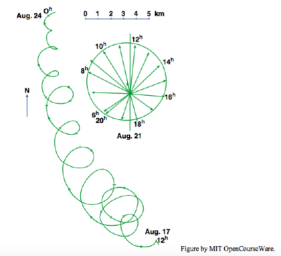
Figure \(\PageIndex{1}\) shows the track of a tracer in an inertia current that was measured over a period of about a week in the Baltic Sea (Gustafson and Kullenberg, 1933). The periods of the loops match the theoretical inertia period for that latitude very closely. There is net translation of the marker because the inertia current was superimposed on a larger-scale current of some other kind. Note that the size of the inertia circles decreases with time, presumably because the current slowed down because of friction.