6.5: Combined Flow (Waves plus Current)

Introduction

It is common, in lakes and in the ocean, for currents and waves to coexist. Such a flow, involving both waves and a current, is called combined flow. In the interior of the current, far away from the bottom boundary, the waves superimpose upon the current a wholesale oscillatory motion of the water that does not affect in any substantial way the structure of turbulence in the current, because very little shear is introduced into the fluid. Near the bottom, however, in the bottom boundary layer, the oscillatory wave motion and the unidirectional current interact in complex ways, with important consequences for sediment entrainment and movement. Such a boundary layer is called a combined-flow boundary layer or a wave-plus-current boundary layer.

Varieties of Combined Flow

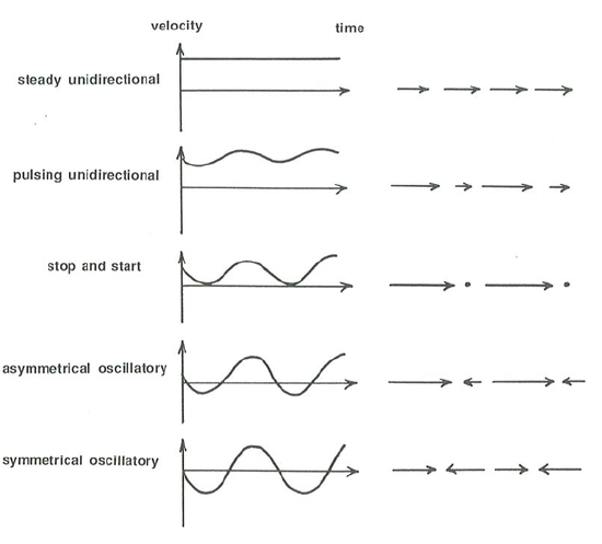
The simplest of combined flows are those involving a train of waves of the “wave tank” variety (with only one wave component, with a single period and a single direction) and the direction of wave propagation is the same as the direction of the current. Then you can imagine a range of combined flows, with one end member being a symmetrical purely oscillatory flow and the other end member being a current without superimposed waves (Figure \(\PageIndex{1}\)). In the range for which the oscillatory flow speed is greater than the unidirectional flow speed, the water elements oscillate but undergo a net shift in position. In the range for which the unidirectional flow speed is greater than the oscillatory flow speed, the water elements move in one direction only but at time-varying speed. The “middle” case is that of a stop–start movement.

Figure \(\PageIndex{1}\): The range of combined flows, when the orientations of the unidirectional component and the oscillatory component are the same.

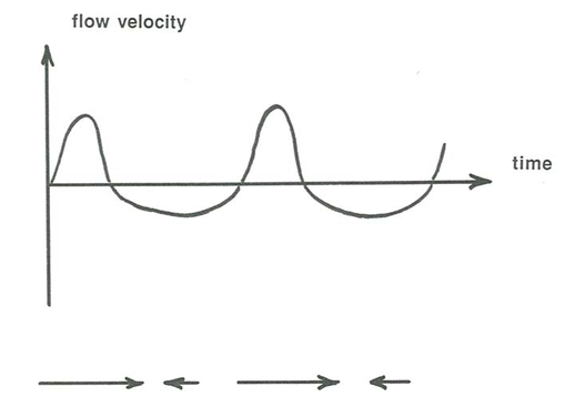
Just to complicate matters further, the asymmetry in the maximum forward and backward velocities in oscillation-dominated combined flow is not the only way that such a velocity asymmetry is produced: it can exist even in purely oscillatory flow for which the forward stroke is at a higher velocity but for a shorter time, and the backward stroke is at a lower velocity but for a longer time (Figure \(\PageIndex{2}\)). the net water movement is still zero, but there is asymmetry in the velocities, and, if the waves are moving sediment, an even greater asymmetry in sediment transport. Such asymmetrical purely oscillatory flow develops when shallow-water waves are propagating into shallower water (that is called shoaling).

Figure \(\PageIndex{2}\): Time history of flow velocity in asymmetrical purely oscillatory flow.

Of course, the range of combined flow described above are a special case, because there can be any angle between the direction of wave propagation and the direction of the current, from zero degrees to ninety degrees. Most of the experimental work on combined flow has been done in the zero-degree case, because that is by far the easiest to set up in the laboratory. In the natural environment, however, the zero-degree case is the exception rather than the rule. Some thought on your part should convince you that the non-zero-degree case involves water movements that are either looping or zigzag, depending upon whether the flow is oscillation-dominated or current-dominated, respectively.

Matters are considerably more complicated when the waves are spectral waves, with more than one component. A bit of elementary physics might help here to guide your thinking. When two sinusoidal oscillations in a horizontal plane, with the same frequency, are combined, the resulting trajectories of material particles describe an ellipse. If, however, the frequencies are different, the trajectories acquire a more complicated, but infinitely repeating, pattern, called Lissajous figures These figures are complexly looping, but they are infinitely repeating, tracing out the same trajectory over and over again, always within the confines of a rectangular box defined by the amplitudes of the two oscillations. (Try googling “Lissajous figures” on the Internet to see some engaging animations.) Such figure simulate what the bottom water movements would be under the action of two wave components with different periods and amplitudes.

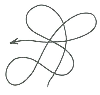
Matters become more complicated when there are three or more oscillatory components, with different orientations and frequencies. Then the particle trajectories appear totally irregular and non-repeating (see Figure \(\PageIndex{3}\), which is fake but it gives you the idea). Such would be the nature of bottom water movements in purely oscillatory flow produced by spectral waves for which more than one component contributes to the bottom water movement. Keep in mind that all of this is before a current is superimposed on the oscillatory motion.

Figure \(\PageIndex{3}\): Cartoon to give you some idea of what the trajectories of near-bottom water elements would be in the case of three or more oscillatory components, with different orientations and frequencies.

The effects of this most general case of combined flow on sediment movement has, to my knowledge a least, been little studied in the laboratory, owing to the great difficulty in arranging for such flows, but sediment movement under such flows in common natural environments like lakes and the shallow ocean must be more the rule than the exception.

What helps to save sedimentationists from this morass of complexity is the low-pass-filter effect of the water column, mentioned earlier: even in the case of a broadly two-dimensional wave spectrum, the bottom water movements are likely to be dominated by only the strongest component(s), thereby making the water movements more like the simpler cases discussed above. At times when the wave spectrum is undergoing major adjustments to the changing direction of strong winds, however, the more general case is likely to be important.

The Combined-Flow Boundary Layer

In combined flows, the boundary layer consists of a wave boundary layer, immediately adjacent to the bottom, commonly some tens of centimeters thick if the bottom is sufficiently rough as to cause the wave boundary layer to be turbulent, and a much thicker current boundary layer, extending upward for tens of meters (see Chapter 7 for more on current boundary layers in large-scale natural environments influenced by the Earth’s rotation.) In other words, the wave boundary layer is embedded in the lowermost part of the current boundary layer. Such boundary layers are called combined-flow boundary layers or wave–current boundary layers. Such boundary layers are the rule during storms in the shallow ocean, over continental shelves, and as such they are a key aspect of continental-shelf sediment transport.

A simple-minded approach to the structure of wave–current boundary layers would be to simply add the time-varying velocity of a wave boundary layer to the unidirectional-flow velocity profile. The problem is that such an approach does not take into account a substantial element of nonlinearity, as follows. Within the wave boundary layer, the superimposition of the current causes the forward stroke of the oscillatory bottom water motion to be of greater velocity than the backward stroke. You learned back in Chapter 4 that, for fully developed turbulent flow (sufficiently large Reynolds number) the flow resistance goes approximately as the square of the velocity—so you should expect the time-average boundary shear stress beneath the wave–current boundary layer to be greater than what it would be for the given current without the accompanying waves. You should expect that the characteristics of the turbulence within the wave boundary layer would be much different from the purely oscillatory case. Above the wave boundary layer, however, the turbulence is unaffected by the presence of the wave boundary layer below: there, you can indeed think in terms of a bodily back-and-forth oscillatory motion being superimposed on the unidirectional current. One way of expressing this is that the wave boundary layer “sees” this region or layer of the flow—within the current boundary layer but above the wave boundary layer—as the interior of the flow. If you could observe the details of the flow in this layer while moving your head in orbits that match the oscillatory component of the flow, they would look the same as if there were no oscillatory component to the flow.

The velocity profile in the combined flow above the wave boundary layer is different from that of a purely unidirectional current, though, because the “anchoring” effect on the profile in the region of the flow nearest the bed is different. Do you recall from Chapter 4 (see Figure 4.8.1 in particular) how, at any given level above the bed in a unidirectional current the slope of the law-of- the-wall velocity profile is the same for dynamically rough flow as for dynamically smooth flow but the actual velocity is smaller, because of the greater boundary resistance in rough flow? In a wave–current boundary layer the presence of the wave boundary layer has an effect of the same kind: the slope of the velocity profile, a reflection of the turbulence structure of the current, is the same as for a purely unidirectional current, but the velocity is smaller because of the greater flow resistance at the bottom of the wave boundary layer. This is shown clearly in Figure \(\PageIndex{4}\): look at the two curves in the left-hand part of the graph, and you will see that at a given elevation the velocity is smaller for the combined flow than in the purely unidirectional flow.

Figure \(\PageIndex{4}\): Velocity profiles in purely unidirectional flow, purely oscillatory flow, and combined flow. The red dots are for purely unidirectional flow; the blue squares are for purely oscillatory flow; and the green circles are for combined flow. The two curves on the left show the unidirectional velocity component, and the curves on the right show the oscillatory velocity component. (From Nielsen, 1992, p. 62.)

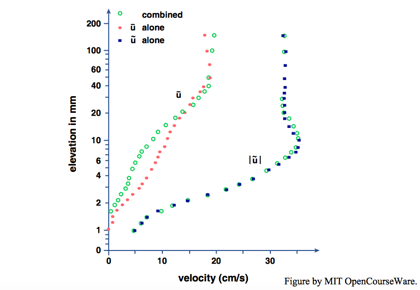
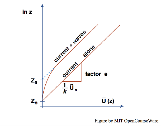
It is also clear from Figure \(\PageIndex{4}\) that the oscillatory velocity in the wave boundary layer in a combined flow is not much different from the oscillatory velocity in the wave boundary layer of a purely oscillatory flow, at least for flows in which the oscillatory component is larger than the unidirectional component. The bottom line, therefore, is that the velocity profile in the wave boundary layer is not greatly changed by the addition of a current, but the velocity profile in the flow above the wave boundary layer is substantially different than in a purely unidirectional flow (Figure \(\PageIndex{5}\)).

Figure \(\PageIndex{5}\): How the addition of an oscillatory component of the flow changes the velocity profile of the unidirectional component of the flow. (From Nielsen, 1992, p. 79.)

References

• Nielsen, P., 1992, Sea Bed Mechanics.
• Schlichting, H., 1960, Boundary Layer Theory: New York, McGraw-Hill, 647 p.