
5.5: The Hydraulic Jump
- Page ID
- 4180

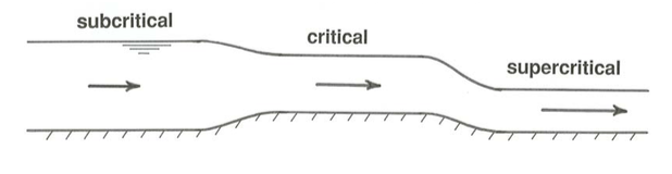
We still have not milked the positive-step example, as arranged in Figure 5.4.6, for all the insight it affords. We made the implicit assumption that the flow coming from upstream had a combination of depth and velocity corresponding to the given \(q\) that was the outcome of the particular gentle channel slope that exists for a long distance upstream; see the earlier section on uniform flow. The combination of slope, discharge per unit width, and bed roughness was such as to provide subcritical flow at that \(d\) and \(U\). We should expect that the flow would like to settle back to that same subcritical condition, somewhere far downstream of the step. But you have just seen that for a sufficiently high step— just high enough for the flow to attain the condition of critical flow, but not so high as to change the upstream flow—the flow for some distance downstream of the step is supercritical. How, then, does the flow pass from being supercritical, just downstream of the step, to subcritical far downstream? The answer is that commonly in situations like this the change from supercritical to subcritical is abrupt, in the form of what is called a hydraulic jump, rather than gradual.
Hydraulic jumps are a striking feature of open-channel flow. You have all seen them, if only in your kitchen sink. You turn the faucet on full force, and the descending jet impinges on the bottom of the sink to form a thin, fast-moving sheet of water, with supercritical depth and velocity, that spreads out in all directions. But at a certain radius from the point of impact of the jet, which depends on the force of the down-flowing jet, the flow jumps up to a deeper and slower flow as it moves toward the drain. The jump is in the form of a steep and nearly stationary front accompanied by strong turbulence (Figure \(\PageIndex{1}\)). Another situation in which a hydraulic jump commonly forms is downstream of a change from a relatively steep channel slope, with which supercritical flow is associated, to a relatively gentle channel slope, over which a uniform flow would be subcritical. If the change in slope is sufficiently rapid, the transition from supercritical flow to subcritical flow is in the form of a hydraulic jump rather than a smooth change in depth and velocity.
The nature of the hydraulic jump cannot be accounted for by use of the energy equation, because there is a substantial dissipation of energy owing to the turbulence associated with the jump; we need to appeal instead to conservation of momentum.
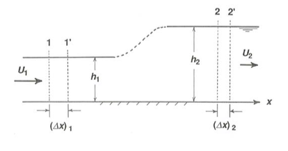
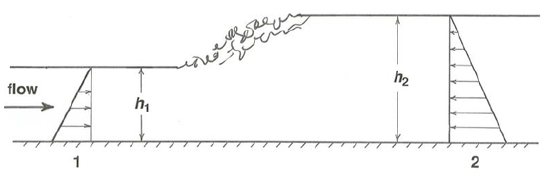
Figure \(\PageIndex{1}\) is a cross-section view of the flow from upstream of the hydraulic jump to downstream of it. Look at a block of the flow bounded by imaginary vertical planes at cross sections \(1\) and \(2\). The distributions of hydrostatic pressure forces are shown on the upstream and downstream faces of the block. You would have to locate section \(2\) quite a distance downstream of the jump, because it takes a long distance for the downstream flow to become organized. In the absence of any submerged obstacle to the flow between sections \(1\) and \(2\), the only streamwise forces on the fluid in the block are the pressure forces on the upstream and downstream faces; the hydraulic jump itself exerts no force on the flow. To see the effect of these forces, we need to do some momentum bookkeeping for use in Newton’s second law, \(F = ma\). For that purpose, look at Figure \(\PageIndex{2}\), a slight redrawing of Figure \(\PageIndex{1}\).
In a short time interval \(\Delta t\), the block of fluid moves downstream from positions \(1\) and \(2\) to positions \(1^{\prime}\) and \(2^{\prime}\). In that time it has lost momentum equal to that of the fluid that was between sections \(1\) and \(1^{\prime}\). That momentum, written per unit flow width (remember that the channel is of the same width from upstream to downstream of the hydraulic jump) is \(\left[\rho d_{1}(\Delta x)_{1}\right] U_{1}\), where \(U_{1}\) is the mean velocity at section \(1\). This can be expressed slightly differently, keeping in mind that \(U_{1} = (\Delta x)_{1} / \Delta t\) and \(q = Ud\), as \(\rho d_{1} U_{1}^{2} \Delta t\), or \(\rho q U_{1} \Delta t\). This can be written in still another form by eliminating \(U_{1}\) by use of the relationship \(q = Ud\) again: \(\left(q^{2} \rho / d_{1}\right) \Delta t\). Likewise, during \(\Delta t\) the fluid block has gained momentum equal to that of the fluid that has moved in to occupy the volume between sections \(2\) and \(2^{\prime}\): \(\left(q^{2} \rho / d_{2}\right) \Delta t\). The change in momentum as the fluid block moves from position \(1–2\) to position \(1^{\prime}–2^{\prime}\) is then
\[\left(\frac{q^{2} \rho}{h_{1}}\right) \Delta t-\left(\frac{q^{2} \rho}{h_{2}}\right) \Delta t \label{5.15} \]
or
\[\left(\frac{q^{2} \rho}{h_{1}}-\frac{q^{2} \rho}{h_{2}}\right) \Delta t \label{5.16} \]
The time rate of change of momentum of the fluid block is then obtained by dividing by the time interval \(\Delta t\):
\[\frac{q^{2} \rho}{h_{1}}-\frac{q^{2} \rho}{h_{2}} \label{5.17} \]
By Newton’s second law, we can set this rate of change of momentum equal to the net streamwise force on the fluid block, \(F_{1}\) (acting in the downstream direction) minus \(F_{2}\) (acting in the upstream direction). The linear distribution of hydrostatic pressure forces on the upstream and downstream faces of the fluid block make it easy to find the resultant forces \(F_{1}\) and \(F_{2}\):
\[F_{1}=\int_{0}^{h_{1}} \rho g y d y=\frac{1}{2} \rho g h_{1}^{2} \label{5.18} \]
and likewise \(\mathrm{F}_{2}=(1 / 2) \rho \mathrm{g} d_{2}^{2}\). The net force on the fluid block is then
\[F_{1}-F_{2}=\frac{\rho g h_{1}^{2}}{2}-\frac{\rho g h_{2}^{2}}{2} \label{5.19} \]
Finally, setting this net force equal to the rate of change of momentum,
\[\frac{q^{2} \rho}{h_{1}}-\frac{q^{2} \rho}{h_{2}}=\frac{\rho g h_{1}^{2}}{2}-\frac{\rho g h_{2}^{2}}{2} \label{5.20} \]
We can massage this a bit to put it into a form that is more convenient for our purposes by rearranging and dividing through by \(\rho g\):
\[\left(\frac{q^{2}}{g h_{1}}+\frac{h_{1}^{2}}{2}\right)-\left(\frac{q^{2}}{g h_{2}}+\frac{h_{2}^{2}}{2}\right)=0 \label{5.21} \]
What is commonly done is to define a quantity
\[M=\frac{q}{g d}+\frac{d^{2}}{2} \label{5.22} \]
called the momentum function. Then Equation \ref{5.21} boils down to \(M_{1} - M_{2} = 0\), which says that the momentum function does not change through the transition, provided that no streamwise forces other than the hydrostatic pressure forces (like resistance forces exerted by obstacles in the channel bottom) act on the fluid block.
Just as with the specific energy in an earlier section, we can plot a useful graph of the momentum function \(M\) against the flow depth d (Figure 5-15). And just as with the specific-energy diagram (Figure 5.2.1), you can verify the shape of the curve in Figure \(\PageIndex{3}\) by assuming a value for \(q\), choosing some values for \(d\), and computing the corresponding values of \(M\); in this case, however, there is no unrealistic limb of the function below the \(d = 0\) axis. There is a family of curves, of the general shape shown in Figure \(\PageIndex{3}\), one for each value of discharge per unit width \(q\). As with the specific-energy diagram, all points on the upper limb of each curve, above the point of vertical tangent, represent supercritical flow, and all points on the lower limb, below the point of vertical tangent, represent subcritical flow.
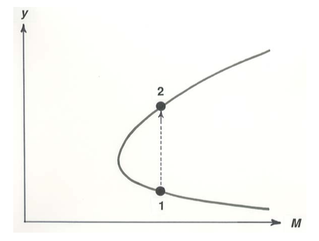
Now we have the tools to predict the height of the hydraulic jump. We start at point \(1\) on the lower, supercritical limb of the curve in Figure \(\PageIndex{3}\), and jump up to point \(2\), at the same value of \(M\) but on the upper, subcritical limb, corresponding to the deeper, subcritical flow downstream of the hydraulic jump. You can see that the closer to the critical condition the upstream supercritical flow is, the smaller is the height of the hydraulic jump to subcritical flow, represented by the vertical distance between the respective points of intersection of the \(M =\) constant vertical line with the two limbs of the curve in Figure \(\PageIndex{3}\).
Note
Just as the shapes of the curves in the family of curves with q as the parameter in Figure \(\PageIndex{3}\) differ from the shapes of the corresponding curves in Figure 5.2.1, the specific-head diagram, so do the equations for the condition of critical flow—but that need not concern us here. You yourself can take the one further step, the same as for the specific-head diagram, to find the shape of the curve for critical flows in Figure \(\PageIndex{2}\), the momentum-function diagram.
Finally, one incidental note is in order. The subcritical flow downstream of the jump, which emerges from the considerations above, is not exactly of the same depth and velocity as the subcritical uniform flow that is ultimately attained far downstream of the step; there is some slow further adjustment to that condition.