
4.6: Flow Resistance
- Page ID
- 4174

Introduction
This section takes account of what is known about the mutual forces exerted between a turbulent flow and its solid boundary. You have already seen that flow of real fluid past a solid boundary exerts a force on that boundary, and the boundary must exert an equal and opposite force on the flowing fluid. It is thus immaterial whether you think in terms of resistance to flow or drag on the boundary.
Forces Exerted by a Flow on its Boundary
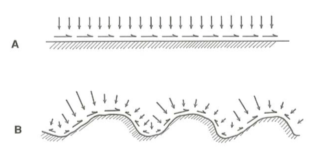
What is the physical nature of the mutual force between the flow and the boundary? Remember that at every point on the solid boundary, no matter how intricate in detail the geometry of that boundary may be, two kinds of fluid forces act: pressure, acting normal to the local solid surface at the point, and viscous shear stress, acting tangential to the local solid surface at the point.
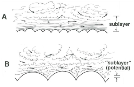
If the boundary is physically smooth (Figure \(\PageIndex{1}\)A) the downstream component of force the fluid exerts on the boundary can result only from the action of the viscous shear stresses, because the pressure forces can then have no component in the direction of flow. But the boundary may be strongly uneven or rough on a small scale at the same time it is planar or smoothly curving on a large scale; this unevenness or roughness might involve arrays of various kinds of bumps, corrugations, protuberances, or particulate masses. Most natural flows, and many in engineering practice also, like canals and corroded pipes, have physically rough boundaries. Then the picture is more complicated (Figure \(\PageIndex{1}\)B), because there is a downstream component of pressure force on the boundary in addition to a downstream component of viscous force: just as with the drag on spheres, considered in Chapters 2 and 3, if roughness elements are present on the boundary, local pressure forces are greater on the upstream sides than on the downstream sides, so each element is subjected to a resultant pressure force with a component in the downstream direction.
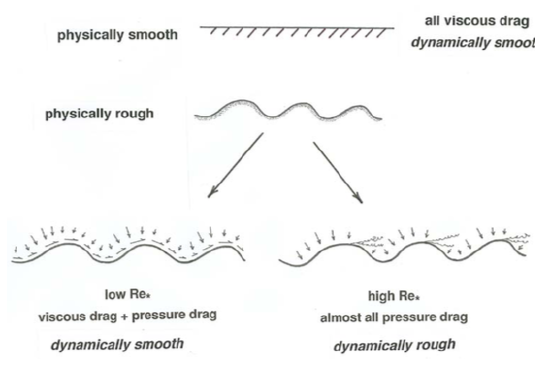
The details of pressure forces on roughness elements are complicated, because they depend not only on a Reynolds number based on the size of the roughness elements and the local velocity of flow around the elements (in generally the same way that the pressure forces depend on a Reynolds number in the case of unbounded and uniform flow around a sphere, as was discussed in earlier chapters), but also on the shape, arrangement, and spacing of the elements. Qualitatively, however, the picture is clear (Figure \(\PageIndex{2}\)): at low Reynolds numbers the pressure force on an element is of the same order as the viscous force, as in creeping flow past a sphere, whereas at higher Reynolds numbers the pressure forces are much greater than the viscous forces, as in separated flow past a sphere.
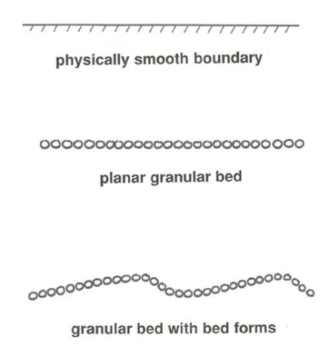
The sum of all the forces on individual roughness elements on the boundary (or, in the case of a physically smooth boundary, the sum of the viscous shear stresses at all points of the boundary) constitutes the overall drag on the boundary, or conversely the overall resistance to the flow; when expressed as force per unit area this boundary resistance is called the boundary shear stress, denoted by \(\tau_{\text{o}}\) (usually pronounced tau-zero or tau-naught). It is important to remember that \(\tau_{\text{o}}\) refers not to the viscous shear stress at any given point on the flow boundary—which seems to fit the description of “boundary shear stress” perfectly!—but to the average force per unit area, viscous forces plus pressure forces, over an area of the boundary large enough that the variations in local forces from point to point are suitably averaged out. That means an area many times the size of the individual roughness elements (Figure \(\PageIndex{3}\)).
It is worth considering at this point how the boundary shear stress \(\tau_{\text{o}}\) is actually measured in pipes and channels. Direct measurement is difficult even in the laboratory: mechanical shear plates set flush with the boundary tend to cause some disturbance to the flow because of the inevitable gap or step at the edges. Hot-film sensors, which measure the shear at the fluid–solid interface indirectly via the conductive heat transfer from a heated solid surface, get around this problem nicely for smooth boundaries, but they do not work well for rough boundaries, especially when the roughness elements are in motion, like sediment grains. Direct measurement under field conditions has been limited.
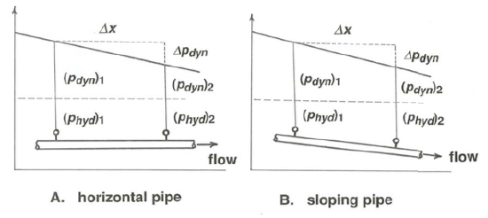
Fortunately, there are other ways of measuring the boundary shear stress. In a horizontal closed conduit you can measure the downstream pressure gradient just by installing two pressure gauges some distance apart, reading the pressure drop, and dividing by the distance between the gauges (Figure \(\PageIndex{4}\)A). Then you can use an equation, analogous to Equation 4.2.1, that relates the boundary shear stress to the pressure gradient. If the conduit is not horizontal, be sure to subtract out the difference in hydrostatic pressure between the two stations, so that you are left with the dynamic pressure (Figure \(\PageIndex{4}\)B). In a steady and uniform channel flow you can use Equation 4.2.1, the resistance equation for channel flow, to find \(\tau_{\text{o}}\) without concern for the internal details of the flow simply by measuring the slope of the water surface; although not always a simple matter, this is possible in both field and laboratory with the proper surveying equipment. The problem is that the value of \(\tau_{\text{o}}\) obtained in this way is the average around the wetted perimeter of the cross section, so it is not exactly the same as the boundary shear stress at any particular place on the wetted perimeter. Moreover, if the channel flow is not uniform—if the depth and velocity vary from section to section—then Equation 4.2.1 holds only approximately, not exactly; the error introduced depends on the degree of nonuniformity.
Another method of finding \(\tau_{\text{o}}\), suitable only for laboratory experiments with smooth flow, is to measure the velocity profile within the viscosity-dominated zone of flow very near the boundary, using various techniques, in order to determine velocity gradient at the boundary, which by Equation 1.3.6 is proportional to \(\tau_{\text{o}}\). One serious problem here is that the viscous sublayer is very thin, necessitating that the measuring device be extremely small for accurate results. Another problem is that this technique is not workable in situations where the roughness elements are larger than the potential thickness of the viscous sublayer—and that is true of most sediment-transporting flows of interest in natural environments.
Finally, you will see presently, after considering velocity profiles in turbulent flow, that \(\tau_{\text{o}}\) can also be found indirectly in both rough and smooth flow by means of less demanding measurement of the velocity profile through part or all of the flow depth. This last method is the most useful of all.
Smooth Flow and Rough Flow
Two fundamentally different but intergrading cases of turbulent boundary-layer flow can be distinguished by comparing the thickness of the viscous sublayer and the height of granular roughness elements. (What I will say here is for sand-grain roughness, but the situation is about the same for close-packed roughness of any geometry.) The roughness elements may be small compared to the thickness of the sublayer and therefore completely enclosed within it (Figure \(\PageIndex{5}\)A). Or they may be larger than what the sublayer thickness would be for the given flow if the boundary were physically smooth rather than rough (Figure \(\PageIndex{5}\)B). In the latter case, flow over and among the roughness elements is turbulent, and the structure of this flow is dominated by effects of turbulent momentum transport. There can then be no overall viscous sublayer in the sense described in an earlier section, although, as noted earlier, a thin viscosity- dominated zone with thickness much smaller than the roughness size must still be present at the very surfaces of all of the roughness elements. In the transitional case the roughness elements poke up through a viscous sublayer that is of about the same thickness as the size of the elements.
If, in flow over a rough bed, the viscous-sublayer thickness is much greater than the size of the roughness elements, the overall resistance to flow turns out to be almost the same as if the boundary were physically smooth; such flows are said to be dynamically smooth (or hydraulically or hydrodynamically or aerodynamically smooth), even though they are in fact geometrically rough. (Obviously, flow over physically smooth boundaries is also dynamically smooth.) This is a consequence of the argument, introduced above, that if the Reynolds number of flow around individual roughness elements is small, as must be the case if the elements are much smaller than the viscous sublayer, pressure forces and viscous forces are of about the same magnitude, so that the presence of roughness makes little difference in the overall resistance to flow. If the elements are much larger than the potential thickness of the viscous sublayer, however, Reynolds numbers of local flow around the elements are large enough that pressure forces on the elements are much larger than viscous forces, and then the roughness has an important effect on flow resistance. Such flows are said to be dynamically rough. There is an intermediate range of conditions for which the flow is said to be transitionally rough.
It is convenient to have a dimensionless measure of distance from the boundary that can be used to specify the thicknesses of the viscous sublayer and the buffer layer. Assume for this purpose that the dynamics of flow near the boundary is controlled only by the shear stress \(\tau_{\text{o}}\) and the fluid properties \(\rho\) and \(\mu\). This should seem at least vaguely reasonable to you, in that the dynamics of turbulence and shear stress in the viscous sublayer and buffer layer are a local phenomenon related to the presence of the boundary but not much affected by the weaker large-scale eddies in the outer layer. There will be more on this in the later section on velocity profiles. You can readily verify that the only possible dimensionless measure of distance \(y\) from the boundary would then be \(\rho^{1 / 2} \tau_{0}^{1 / 2} y / \mu\), often denoted by \(y^{+}\). A similar dimensionless variable \(\rho^{1 / 2} \tau_{0}^{1 / 2} D / \mu\), involving the height \(D\) of roughness elements on the boundary, can be derived by the same line of reasoning about variables important near the boundary. This latter variable is called the boundary Reynolds number or the roughness Reynolds number, often denoted by \(\text{Re}_{*}\).
The dimensionless distance \(y^{+}\) and the roughness Reynolds number \(\text{Re}_{*}\) can be written in a more convenient and customary form by introduction of two new variables. The quantity \(\left(\tau_{0} / \rho\right)^{1 / 2}\), usually denoted by \(u_{*}\) (pronounced u-star), has the dimensions of a velocity; it is called the shear velocity or the friction velocity. Warning: \(u_{*}\) is not an actual velocity; it is a quantity involving the boundary shear stress that conveniently has the dimensions of a velocity. The quantity \(\mu /\rho\), which you may have noticed commonly appears in Reynolds numbers, is called the kinematic viscosity, denoted by \(ν\). The word kinematic is used because the dimensions of \(ν\) involve only length and time, not mass. If \(y^{+}\) as defined above is rearranged slightly it can be written \(u_{*}y/ν\) and the roughness Reynolds number can be written \(u_{*} D/ν\).
When expressed in the dimensionless form \(y^{+}\), the transition from the viscous sublayer to the buffer layer is at a \(y^{+}\) value of about \(5\), and the transition from the buffer layer to the turbulence-dominated layer is at a \(y^{+}\) value of about \(30\). These transition values are about the same whatever the values of boundary shear stress τo and fluid properties \(\rho\) and \(\mu\); this confirms the supposition made above that over a wide range of turbulent boundary-layer flows the variables \(\tau_{\text{o}}\), \(\rho\), and \(\mu\) suffice to characterize the flow near the boundary. These values are known not from watching the flow but from plots of velocity profiles, as will be discussed presently.
The relative magnitude of the viscous-sublayer thickness and the roughness height \(D\) can be expressed in terms of the roughness Reynolds number \(u_{*}D/ν\). To see this, take the top of the viscous sublayer to be at \(u_{*} \delta_{v} / v \approx 5\), meaning that \(\delta_{v} \approx 5 v / u_{*}\) is the distance from the boundary to the top of the viscous sublayer. Here I have replaced \(y\) by \(\delta_{v}\), the thickness of the viscous sublayer. The ratio of particle size to sublayer thickness is then \(D / \delta_{v} \approx\left(u_{*} D / v\right) / 5\). In other words, sublayer thickness and particle size are about the same when the roughness Reynolds number has a value of about \(5\). (But remember that if the roughness elements are this large or larger, there is no well developed viscous sublayer in the first place.) Another way of looking at this is that we can compare the particle size \(D\) with \(v/ u_{*}\), a quantity with dimensions of length called the viscous length scale, which is proportional to the thickness of the viscous sublayer.
The limits of smooth and rough flow can also be specified by values of the roughness Reynolds number. The upper limit of smooth flow is associated with the condition that the height of the viscous sublayer is about equal to that of the roughness elements. As noted above, at the top of the viscous sublayer \(y^{+}=u_{*} \delta_{v} / v \approx 5\), so the upper limit of roughness Reynolds numbers for smooth flow should be \(u_{*} D / \nu \approx 5\), and in fact the value of \(5\) is in good agreement with results based on both boundary resistance and velocity profiles. Likewise, the lower limit of roughness Reynolds numbers for fully rough flows is found to be about \(60\). It is between these values \(\left(5<u_{*} D / v<60\right)\) that the flow is said to be transitionally rough.
Some further discussion of smooth and rough flow can be found in the latter part of this chapter in the section on velocity profiles.
Dimensional Analysis of Flow Resistance
One circumstance that tends to make the standard treatments of flow resistance in fluid-dynamics textbooks seem more complicated than they really are is that the details of the equations for flow resistance (although not their general form) depend not only on the boundary roughness but also on the overall geometry of the flow. On the one hand, the flow may be a turbulent boundary layer growing into a free stream; on the other hand, it may be a fully established turbulent boundary layer that occupies all of a conduit or channel. In terms of flow mechanics in the boundary layer itself, these two kinds of flow can be treated together. In the latter case any number of boundary geometries are possible. The classic experiments on flow resistance were made using circular pipes with inside surfaces coated with uniform sand, and not much systematic work has been done on channel flow. The discussion here focuses on pipe flow, with the understanding that both the principles and the general form of the results are the same for any steady uniform flow whatever the boundary geometry.
In common with other aspects of turbulent boundary-layer flow, there is no theory we can draw on to find relationships for flow resistance. It is therefore again natural to start with a dimensional analysis of resistance to flow through a circular pipe or tube (Figure \(\PageIndex{6}\)) in order to develop a framework in which experimental data can provide dimensionless relationships that are expressible in the form of essentially empirical equations that are valid in certain ranges of flow.
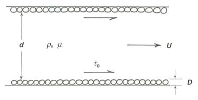
Which variables must be specified in order that the boundary shear stress \(\tau_{\text{o}}\) can be fully characterized or determined? Pipe diameter \(d\) and mean flow velocity \(U\) are important because they affect the rate of shearing in the flow, both directly and through their effect on the structure of turbulence. Viscosity \(\mu\) is obviously important because of its role in determining viscous shear stress at the boundary. Fluid density \(\rho\) is important because if the flow is turbulent there must be local fluid accelerations. Finally, the size \(D\) of boundary roughness elements may affect the turbulent forces and motions near the boundary. There are thus two important length scales in the problem of flow resistance: pipe diameter and roughness height. We will have to assume that shape, spacing, and arrangement of the roughness elements are either always the same or, if variable, are of secondary importance in determining flow resistance. Neither assumption is justified, but they form a good place to start. Never mind that if the boundary is rough there is some haziness about where the position of the wall should be taken in defining the pipe diameter; at least with respect to flow resistance, any reasonable choice produces consistent results provided that consideration is limited to geometrically similar roughness.
Assuming that all of the important variables have been included,τo can be viewed as a function of the five variables \(U\), \(d\), \(D\), \(\rho\), and \(\mu\). You should then expect to have a dependent dimensionless variable as a function of two independent dimensionless variables. It should occur to you immediately that one of the independent dimensionless variables can be a Reynolds number based on \(U\) and \(d\), which I will call the mean-flow Reynolds number. The other independent dimensionless variable is most naturally \(d/D\), the ratio of pipe diameter to roughness height. This variable is called the relative roughness. The dependent dimensionless variable, which must involve \(\tau_{\text{o}}\), has exactly the same form and physical significance as the dimensionless drag force or drag coefficient that characterizes the drag on a sphere moving relative to a fluid (Chapter 2), except that here we are dealing with a force per unit area rather than with a force. You can verify that one possible dimensionless variable involving \(\tau_{\text{o}}\) is 8\(\tau_{0} / \rho U^{2}\), and although this is not the only one possible (there are two others; you might at this point try to find them yourself) it is the most useful, and it is the one that is conventionally used. (The factor \(8\) is present for reasons of convenience that need not concern us here.) This dimensionless boundary shear stress is called the friction factor, denoted by \(f\); it is one kind of flow-resistance coefficient.
The functional relationship for flow resistance can thus be written
\[f=\frac{8 \tau_{o}}{\rho U^{2}}=F\left(\frac{\rho U d}{\mu}, \frac{d}{D}\right) \label{4.8} \]
where \(F\) is a function that for turbulent flow has to be ascertained by experiment.
Resistance Diagrams
The relationship expressed in Equation \ref{4.8} can be shown in a two-dimensional graph most easily by plotting curves of \(f\) vs. Reynolds number for a series of values of \(d/D\). Figure \(\PageIndex{7}\) shows a graph of this kind, called a resistance diagram. The data were obtained by Nikuradse (1933) for flows through circular pipes lined with closely spaced sand grains of approximately uniform size. A version of Figure \(\PageIndex{7}\) is shown in just about all books on flow of viscous fluids.
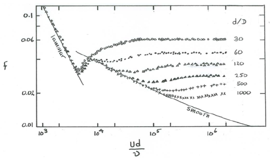
Leaving aside the steeply sloping part of the curve on the far left (it holds for laminar flow in the pipe, for which we have already obtained an exact solution), you see that at fairly low Reynolds numbers the curve off vs. \(\text{Re}\) for any given \(d/D\) in Figure \(\PageIndex{7}\) at first slopes gently down to the right, then breaks away, and finally levels out to a horizontal straight line. The larger the relative roughness \(d/D\) the greater the Reynolds number at which the breakaway takes place. Physically smooth boundaries, for which \(D/d = 0\), follow the descending curve to indefinitely high Reynolds numbers. Flows that plot on this descending curve are those I earlier termed dynamically smooth. Note that flows over physically rough boundaries can be dynamically smooth, provided that \(d/D\) is sufficiently large. If \(\text{Re}\) is fairly small and the pipe is fairly large, \(D\) can be absolutely large—millimeters or even centimeters—in smooth water flows. Flows that plot on the horizontal straight lines to the right are those I called fully rough, and those at intermediate points are those I called transitionally rough. For a given \(d/D\) the flow is smooth at low Reynolds numbers but rough at sufficiently high Reynolds numbers.
Two questions need to be discussed at this point:
- How would the results in Figure \(\PageIndex{7}\) change for kinds of roughness elements different from glued-down uniform sand grains?
- How would the results change for conduits or channels with geometry different from that of a circular pipe?
The answer to both of these questions is that the results are qualitatively the same, provided that the characteristics of the roughness are not grossly different and that the size of the roughness elements remains a small fraction of the conduit diameter or channel depth. The curves are merely shifted slightly in position or differ slightly in shape. To adapt the uniform- sand-roughness results to other kinds of roughness a quantity called the equivalent sand roughness, denoted by \(k_s\), is defined as the fictitious roughness height that would make the results for the given kind of roughness expressible by the same plot as in Figure \(\PageIndex{7}\) for uniform-sand-roughness pipes. And to compare the pipe results with those for conduits or channels with different geometry, it is customary to use the hydraulic radius in place of the pipe radius, although the results cannot be expected to be exactly the same. By applying the definition of hydraulic radius given earlier in this chapter you can verify that for a circular pipe the hydraulic radius specializes to one-fourth the pipe diameter. (You have already seen that for an infinitely wide channel flow the hydraulic radius specializes to the flow depth.)
There is an equivalent way of expressing resistance that is used specifically for open-channel flow. Combining the equation \(\tau_{\text{o}}=(f / 8) \rho U^{2}\) that defines the friction factor \(f\) with the equation \(\tau_{\text{o}}=\rho g d \sin \alpha\) (Equation 4.2.1) for boundary shear stress in steady uniform flow down a plane, eliminating \(\tau_{\text{o}}\) from the two equations, and then solving for \(U\),
\[U=\left(\begin{array}{ll}{\frac{8 g}{f}} & {d \sin \alpha}\end{array}\right)^{1 / 2} \label{4.9} \]
\[U=C(d \sin \alpha)^{1 / 2} \label{4.10} \]
where
\[C=\left(\frac{8 g}{f}\right)^{1 / 2} \label{4.11} \]
Equation \ref{4.11}, which relates mean velocity, flow depth, and slope for uniform flow in wide channels, is called the Chézy equation, after the eighteenth-century French hydraulic engineer who first developed it. The coefficient \(C\), called the Chézy coefficient, is not a dimensionless number like the friction factor \(f\); it has the dimensions \(g^{1 / 2}\). But because \(g\) is very nearly a constant at the Earth’s surface, \(C\) can be viewed as being a function only of \(f\). I have introduced the Chézy \(C\) because it is in common use in work on open-channel flow, but you should understand that it adds nothing new.