4.5: Structure of Turbulent Boundary Layers

Introduction

I have said quite a lot about what turbulence looks like in a general way, but now I need to be more specific about the structure of turbulence in turbulent boundary layers. (Another term I could use instead of turbulent boundary layers is turbulent shear flow: any turbulent flow that involves overall mean shearing, of the fluid, usually on account of the presence of a solid boundary to the flow.)

Many of the important things about turbulence in boundary layers have been known for a long time. Workable techniques for reliable measurement of instantaneous velocities in air were developed half a century ago, in the 1940s and 1950s. Comparable laboratory techniques for water flows became available in the 1960s, and reliable field measurements in water flows became possible later. It is still difficult to make detailed observations of the scales, shapes, motions, and interactions of turbulent eddies, especially the relatively small eddies near the boundary. Only in the last few decades has observational knowledge of the dynamics of near- boundary turbulent structure advanced from the stage of point measurements of velocities and their statistical treatment, to observations of the eddy structure of the turbulent flow as a whole by means of various flow-visualization techniques. Studies on the structure and organization of turbulent fluid motions in boundary layers has become an actively growing branch of fluid dynamics, and has resulted in much deeper understanding of the dynamics of turbulent flows.

In the following section are some of the most important facts and observations on the turbulence structure of turbulent boundary layers—with steady uniform flow down a plane as a reference case, but the differences between this and other kinds of boundary-layer flow lie only in minor details and not in important effects.

Vertical Organization of Flow Structure in Channel Flows

First of all, you should expect the nature of turbulence to vary strongly from surface to bottom in the flow, because the boundary is the place where the vertical turbulent fluctuations must go to zero and where by the no-slip condition the fluid velocity itself must go to zero. You have already seen that the relative contributions of turbulent shear stress and viscous shear stress change drastically in the vicinity of the boundary.

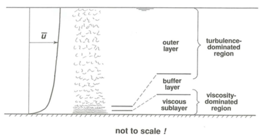
If the bottom boundary is physically smooth, or if it is rough but the height of the roughness elements is less than a certain value to be discussed presently, three qualitatively different but intergrading zones of flow can be recognized (Figure \(\PageIndex{1}\)): a thin viscous sublayer next to the boundary, a turbulence-dominated outer layer occupying most of the flow depth, and a buffer layer between. If the boundary is too rough, the viscous sublayer is missing. Here I will only give a qualitative description of the flow in these layers; in later sections I will show their implications for flow resistance and velocity profiles.

Figure \(\PageIndex{1}\): Division of turbulent open-channel flow into layers on the basis of turbulence structure.

The viscous sublayer is a thin layer of flow next to the boundary in which viscous shear stress predominates over turbulent shear stress. Shear in the viscous sublayer, as characterized by the rate of change of average fluid velocity as one moves away from the wall, is very high, because fast-moving fluid is mixed right down to the top of the viscous sublayer by turbulent diffusion.

The thickness of the viscous sublayer depends on the characteristics of the particular flow and fluid; it is typically in the range of a fraction of a millimeter to many millimeters. You will find out later how to ascertain the viscous-sublayer thickness.

The flow is not strictly laminar in the viscous sublayer because it experiences random fluctuations in velocity. What is important, however, is that because fluctuations in velocity normal to the boundary must decrease to zero at the boundary itself, molecular transport of fluid momentum is dominant over turbulent transport of momentum near the boundary. Fluctuations in velocity very close to the boundary must therefore be largely parallel to the boundary. Fluctuations in shear stress on the boundary itself caused by these fluctuations in velocity can be substantial. The turbulent fluctuations in velocity in the viscous sublayer are the result of advection of eddies from regions farther away from the wall; these eddies are damped out by viscous shear stresses in the sublayer.

When the boundary is physically smooth the thickness of the viscous sublayer can easily be defined, but when the boundary is covered with closely spaced roughness elements (like sediment particles, or corrosion bumps, or densely spaced buildings, or trees and shrubs) with heights greater than the thickness of the viscous sublayer (or, more precisely, what the sublayer thickness would be in the absence of the roughness), then no sublayer is actually present at all, and turbulence extends all the way to the boundary, in among the roughness elements.

Of course, if you zoomed in to look at the boundary even more closely, you would find very thin viscous sublayers right at the surfaces of each of the roughness elements: close enough to any solid surface, the flow has to be dominated by viscous effects. In the preceding paragraph I was talking about the presence or absence of a viscous sublayer over a whole larger area of the boundary, at lateral scales much greater than the individual roughness elements.

The buffer layer is a zone just outside the viscous sublayer in which the gradient of time-average velocity is still very high but the flow is strongly turbulent. Its outstanding characteristic is that both viscous shear stress and turbulent shear stress are too important to be ignored. With reference to Figure \(\PageIndex{1}\) you can see that this is the case only in a thin zone close to the bottom. Very energetic small-scale turbulence is generated there by instability of the strongly sheared flow, and there is a sharp peak in the conversion of mean-flow kinetic energy to turbulent kinetic energy, and also in the dissipation of this turbulent energy; for this reason the buffer layer is often called the turbulence-generation layer. (There will be more on kinetic energy in turbulent flows soon.) Some of the turbulence produced here is carried outward into the broad outer layer of flow, and some is carried inward into the viscous sublayer. The buffer layer is fairly thin but thicker than the viscous sublayer.

The broad region outside the buffer layer and extending all the way to the free surface is called the outer layer. (In pipe flow this is more naturally called the core region.) This layer occupies most of the flow depth, from the free surface down to fairly near the boundary. Here the turbulent shear stress is predominant, and the viscous shear stress can be neglected. Except down near the buffer layer, turbulence in this zone is of much larger maximum scale than nearer the boundary. Because of their large size, the turbulent eddies here are more efficient at transporting momentum normal to the flow direction than are the much smaller eddies nearer the boundary; this is why the profile of mean velocity is much gentler in this region than nearer the bottom. But it turns out that these large eddies contain much less kinetic energy per unit volume of fluid than in the buffer layer. The normal-to-boundary dimension of the largest eddies in this outer layer is a large fraction of the flow depth—but there are smaller eddies too, at a whole range of scales; see a later section for more discussion of eddy scales.

In terms of the relative importance of turbulent shear stress and viscous shear stress, it is convenient to divide the flow in a somewhat different way (Figure \(\PageIndex{1}\)) into a viscosity-dominated region, which includes the viscous sublayer and the lower part of the buffer layer, where viscous shear stress is more important than turbulent shear stress, and a turbulence-dominated region, which includes the outer layer and the outer part of the buffer layer, where the reverse is true. In a thin zone in the middle part of the buffer layer the two kinds of shear stress are about equal. It is worth emphasizing that there are no sharp divisions in all this profusion of layers and regions: they grade smoothly one into another.