3.5: Turbulence

Most of the fluid flows of interest in science, technology, and everyday life are turbulent flows—although there are many important exceptions to that generalization, like the flow of groundwater in the porous subsurface, or the flow of blood in capillaries, or the flow of lubricating fluid in thin clearances between moving parts of a machine, or the flow of that thin, slow-moving sheet of water you see on the paved surface of the shopping-mall parking lot after a rain. Because of the range and complexity of problems in turbulent flow, the approach here will necessarily continue to be selective. The introductory material on the description and origin of turbulence in this section is background for the important topic of turbulent flow in boundary layers in the following section and in Chapter 4. The emphasis in all this material on turbulence is on the most important physical effects. Mathematics will be held to a minimum, although some is unavoidable in the derivation of useful results on flow resistance and velocity profiles in Chapter 4.

What is Turbulence?

It is not easy to devise a satisfactory definition of turbulence. Turbulence might be loosely defined as an irregular or random or statistical component of motion that under certain conditions becomes superimposed on the mean or overall motion of a fluid when that fluid flows past a solid surface or past an adjacent stream of the same fluid with different velocity. This definition does not convey very well what turbulence is really like; it is much easier to describe turbulence than to define it.

Describing Turbulence

My goal in this section is to present to you as clear a picture as possible of what turbulence is like. Suppose that you were in possession of a magical instrument that allowed you to make an exact and continuous measurement of the fluid velocity at any point in a turbulent flow as a function of time. I am calling the instrument magical because all of the many available methods of measuring fluid velocity at a point, some of them fairly satisfactory, inevitably suffer to some extent from one or both of two drawbacks:

1. The presence of the instrument distorts or alters the flow one is trying to measure.
2. The effective measurement volume is not small enough to be regarded as a “point”.

What would your record of velocities look like? Figure \(\PageIndex{1}\) is an example of a record, for the component \(u\) of velocity in the downstream direction. The outstanding characteristic of the velocity is its uncertainty: there is no way of predicting at a given time what the velocity at some future time will be. But note that there is a readily discernible (although not precisely definable) range into which most of the velocity fluctuations fall, and the same can be said about the time scales of the fluctuations.

Figure \(\PageIndex{1}\): Typical record of streamwise instantaneous flow velocity measured at a point in a turbulent channel flow.

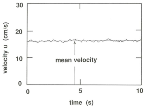
Turbulence measurements present a rich field for statistical treatment. First of all, a mean velocity \(\overline{u}\) can be defined from the record of \(u\) by use of an averaging time interval that is very long with respect to the time scale of the fluctuations but not so long that the overall level of the velocity drifts upward or downward during the averaging time. A fluctuating velocity \(u^{\prime}\) can then be defined as the difference between the instantaneous velocity \(u\) and the mean velocity \(\overline{u}\):

\[u^{\prime}=u-\overline{u} \label{3.17} \]

where the overbar denotes a time average. The time-average value of \(u^{\prime}\) must be zero (by definition!). Now look at the component of velocity in any direction normal to the mean flow direction. You would see a record similar to that shown in Figure \(\PageIndex{1}\), except that the average value would always have to be zero; the normal-to-boundary velocity is usually called \(v\), and the cross-stream velocity parallel to the boundary and normal to flow) is usually called \(w\). Equations just like Equation \ref{3.17} can be written for the components \(v\) and \(w\):

\(v^{\prime}=v-\overline{v}=v\)

\[w^{\prime}=w-\overline{w}=w \label{3.18} \]

A good measure of the intensity of the turbulence is the root-mean- square value of the fluctuating components of velocity:

\(\operatorname{rms}\left(u^{\prime}\right)=\left(u^{\prime 2}\right)^{1 / 2}\)

\[\operatorname{rms}\left(v^{\prime}\right)=\left(v^{\prime 2}\right)^{1 / 2} \label{3.19} \]

\(\operatorname{rms}\left(w^{\prime}\right)=\left(w^{\prime 2}\right)^{1 / 2}\)

These are formed by taking the square root of the time average of the squares of the fluctuating velocities; for those who are familiar with statistical terms, the rms values are simply standard deviations of instantaneous velocities. They are always positive quantities, and their magnitudes are a measure of the strength or intensity of the turbulence, or the spread of instantaneous velocities around the mean. Turbulence intensities are typically something like five to ten percent of the mean velocity \(\overline{u}\) (that is, again in the parlance of statistics, the coefficient of variation of velocity is \(5–10 \%\)).

Several Ways of Analyzing Turbulence

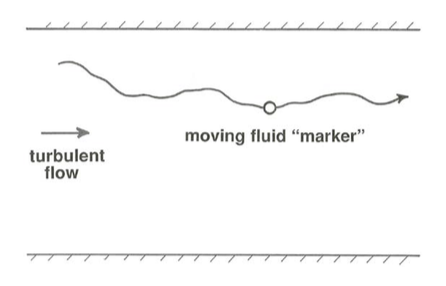
Statistical analysis of turbulence can be carried much further than this. But now suppose that you measured velocity in a different way, by following the trajectories of fluid “points” or markers as they travel with the flow and measuring the velocity components as a function of time (Figure \(\PageIndex{2}\)). It is straightforward, though laborious, to do this sort of thing by photographing tiny neutrally buoyant marker particles that represent the motion of the fluid well and then measuring their travel and computing velocities. Velocities measured in this way, called Lagrangian velocities, are related to those measured at a fixed point, called Eulerian velocities, and the records would look generally similar. The trajectories themselves would be three-dimensionally sinuous and highly irregular, as shown schematically in Figure \(\PageIndex{2}\), although angles between tangents to trajectories and the mean flow direction are usually not very large, because \(u^{\prime}\) is usually small relative to \(\overline{u}\).

Figure \(\PageIndex{2}\): Typical trajectory of a small fluid element or neutrally buoyant marker particle in a turbulent channel flow.

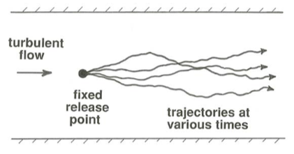
You can also imagine releasing fluid markers at some fixed point in the flow and watching a succession of trajectories traced out at different times (Figure \(\PageIndex{3}\)). Each trajectory would be different in detail, but they would show similar features.

Figure \(\PageIndex{3}\): A series of trajectories of small, neutrally buoyant markers in a turbulent channel flow, all released from the same point.

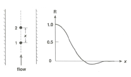
One thing you can do to learn something about the spatial scale of the fluctuations revealed by velocity records like the one in Figure 3.5.1 is to think about the distance over which the velocity becomes “different” or uncorrelated with distance away from a given point (Figure \(\PageIndex{4}\)). Suppose that you measured the velocity component \(u\) simultaneously at two points \(1\) and \(2\) a distance \(x\) apart in the flow and computed the correlation coefficient by forming products of a large number of pairs of velocities, each measured at the same time, taking the average of all the products, and then normalizing by dividing by the \(\text{rms}\) value. If the two points are close together compared to the characteristic spatial scale of the turbulence, the velocities at the two points are nearly the same, and the coefficient is nearly one. But if the points are far apart the velocities are uncorrelated (that is, they have no tendency to be similar), and the coefficient is zero or nearly so. The distance over which the coefficient falls to its minimum value, a bit less than one, before rising again to zero is roughly representative of the spatial scale of the turbulent velocity fluctuations. The gentle minimum is an indication that the distance out from the original point corresponds to adjacent eddies, which tend to have an opposing velocity, hence the minimum. A similar correlation coefficient can be computed for Lagrangian velocities, and correlation coefficients can also be based on time rather than on space.

Figure \(\PageIndex{4}\): Correlation coefficient \(R\) for fluid velocity measured at two points, \(1\) and \(2\), separated by a streamwise (i.e., alongstream) distance \(x\).

Eddies

One of the very best ways to get a qualitative idea of the physical nature of turbulent motions is to put some very fine flaky reflective material into suspension in a well illuminated flow. The flakes tend to be brought into parallelism with local shearing planes, and variations in reflected light from place to place in the flow give a fairly good picture of the turbulence. Although it is easier to appreciate than to describe the pattern that results, the general picture is one of intergrading swirls of fluid, with highly irregular shapes and with a very wide range of sizes, that are in a constant state of development and decay. These swirls are called turbulent eddies. Even though they are not sharply delineated, they have a real physical existence.

The swirly nature of the eddies is most readily perceived when the eye attempts to follow points moving along with the flow; if instead the eye attempts to fix upon a point in the flow that is stationary with respect to the boundaries, fluid elements (if there are some small marker particles contained in the fluid to reveal them) are seen to pass by with only slightly varying velocities and directions, in accordance with the Eulerian description of turbulent velocity at a point.

Each eddy has a certain sense and intensity of rotation that tends to distinguish it, at least momentarily, from surrounding fluid. The property of solid- body-like rotation of fluid at a given point in the flow is termed vorticity. Think in terms of the rotation of a small element of fluid as the volume of the element shrinks toward zero around the point. The vorticity varies smoothly in both magnitude and orientation from point to point. The eddy structure of the turbulence can be described by how the vorticity varies throughout the flow; the vorticity in an eddy varies from point to point, but it tends to be more nearly the same there than in neighboring eddies.

Laminar and Turbulent Flow

At first thought it seems natural that fluids would show a smooth and regular pattern of movement, without all the irregularity of turbulence. Such regular flows are called laminar flows. You will see over and over again in these notes that flows in a given setting or system are laminar under some conditions and turbulent under other conditions. Now that you have some idea of the kinematics of turbulent flow, you might consider what it is that governs whether a given flow is laminar or turbulent in the first place, and what the transition from laminar to turbulent flow is like. Osborne Reynolds did the pioneering work on these questions in the 1880s in an experimental study of flow through tubes with circular cross section (Reynolds, 1883).

Figure \(\PageIndex{5}\): Variables associated with steady flow through a circular tube.

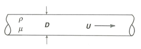
Think first about the variables that must be important in steady flow through a straight circular tube (Figure \(\PageIndex{5}\)). Density \(\rho\) must be taken into account, because of the possibility of turbulent flow in the tube and therefore local fluid accelerations. Viscosity \(\mu\) must be taken into account because it affects the shearing forces within the fluid and at the wall. A variable that describes the speed of movement of the fluid is important, because this governs both fluid inertia and rates of shear. A good variable of this kind is the mean velocity of flow \(U\) in the tube; this can be found either by averaging the local fluid velocity over the cross section of the tube or by dividing the discharge (the volume rate of flow) by the cross-sectional area of the tube. The diameter \(D\) of the tube is important because it affects both the shear rate and the scale of the turbulence. Gravity need not be considered explicitly in this kind of flow because no deformable free surface is involved. By dimensional analysis, as discussed in Chapter 2, the four variables \(U\), \(D\), \(\rho\), and \(\mu\) can be combined into a single dimensionless variable \(\rho U D /\mu\) on which all of the characteristics of the flow, including the transition from laminar to turbulent flow, depend. Reynolds first deduced the importance of this variable, now called the Reynolds number, by considering the dimensional structure of the equation of motion in the way I alluded to briefly at the end of Chapter 2.

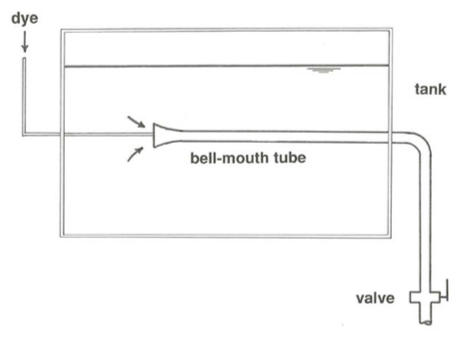
Reynolds made two kinds of experiments. The first, to study the development of turbulent flow from an originally laminar flow, was made in an apparatus like that shown in Figure \(\PageIndex{6}\): a long tube leading from a reservoir of still water by way of a trumpet-shaped entrance section, through which a flow with varying mean velocity could be passed with a minimum of disturbance. Three different tube diameters (\(1/4^{\prime \prime}\), \(1/2^{\prime \prime}\), and \(1^{\prime \prime}; 0.64\), \(1.27\), and \(2.54 \text{cm}\)) and water of two different temperatures, and therefore of two different viscosities, were used. For each combination of \(D\) and \(\mu\), \(U\) was gradually increased until the originally laminar flow became turbulent. The transition was observed with the aid of a streak of colored water introduced at the entrance of the tube.

Figure \(\PageIndex{6}\): Apparatus (schematic) used by Osborne Reynolds in his study of the transition from laminar to turbulent flow in a circular tube.

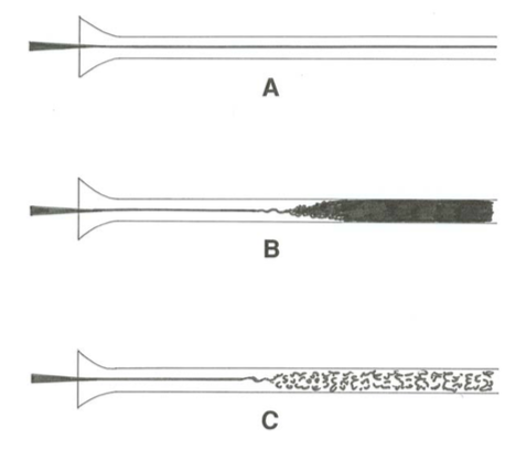
When the velocities were sufficiently low, the streak of color extended in a beautiful straight line through the tube [Figure \(\PageIndex{7}\)A].... As the velocity was increased by small stages, at some point in the tube, always at a considerable distance from the trumpet or entrance, the color band would all at once mix up the surrounding water and fill the rest of the tube with a mass of colored water [Figure \(\PageIndex{7}\)B].... On viewing the tube by the light of an electric spark, the mass of water resolved itself into a mass of more or less distinct curls, showing eddies [Figure \(\PageIndex{7}\)C] - (Reynolds, 1883, p. 942)

Figure \(\PageIndex{7}\): The results of Reynolds’ experiments on the transition from laminar to turbulent flow in a circular tube.

Reynolds found that for each combination of \(D\) and \(U\) the point of transition was characterized by almost exactly the same value of \(\text{Re}\), around \(12,000\). Subsequent experiments have since confirmed this over a much wider range of \(U\), \(D\), \(\rho\), and \(\mu\).

Reynolds suspected that, because the transition from laminar to turbulent flow was so abrupt and the resulting turbulence was so well developed, the laminar flow became potentially unstable to large disturbances at a much lower value of \(\text{Re}\) than he found for the transition when he minimized external disturbances, and in fact he observed that the transition took place at much lower values of \(\text{Re}\) if there was residual turbulence in the supply tank or if the apparatus was disturbed in any way. Similar experiments made with even greater care in eliminating such disturbances have since shown that laminar flow can be maintained to much higher values of \(\text{Re}\), up to about \(40,000\), than in Reynolds’ original experiments.

To circumvent the persistence of laminar flow into the range of \(\text{Re}\) for which it is unstable, Reynolds made a separate set of experiments to study the transition of originally turbulent flow to laminar flow as the mean velocity in the tube was gradually decreased. To do this he passed turbulent flow through a very long metal pipe and gradually decreased the mean velocity until at some point along the pipe the flow became laminar. The occurrence of the transition was detected by measuring the drop in fluid pressure between two stations about two meters apart near the downstream end of the pipe. (It had been known long before Reynolds’ work—and you yourselves will soon be seeing why—that in laminar flow through a horizontal pipe the rate at which fluid pressure drops along the pipe is directly proportional to the mean velocity, whereas in turbulent flow it is approximately proportional to the square of the mean velocity. Thus, although Reynolds could not see the transition he had a sensitive means of detecting its occurrence.) Again many different combinations of \(D\) and \(\mu\) were used, and in every case the transition from turbulent to laminar flow occurred at values of \(\text{Re}\) close to \(2000\). This is the value for which laminar flow can be said to be unconditionally stable, in the sense that no matter how great a disturbance is introduced, the flow always reverts to being laminar.

Origin of Turbulence

Mathematical theory for the origin of turbulence is intricate, and only partly successful in accounting for the transition to turbulent flow at a certain critical Reynolds number. One of the most successful approaches involves analysis of the stability of a laminar flow against very small-amplitude disturbances. The mathematical technique involves introducing a small wavelike disturbance of a certain frequency into the equation of motion for the flow and then seeing whether the disturbance grows in amplitude or is damped. The assumption is that if the disturbance tends to grow it will eventually lead to development of turbulence.

Although a satisfactory explanation would take us off the track at this point, in laminar flow there is a tendency for a wave-shaped distortion like the one in Figure \(\PageIndex{8}\) to be amplified with time: applying the Bernoulli equation along the streamlines shows that fluid pressure is lowest where the velocity is greatest in the region of crowded flow lines, and highest where the velocity is smallest in the region of uncrowded flow lines, and the resulting unbalanced pressure force tends to accelerate the fluid in the direction of convexity and thereby accentuate the distortion. But at the same time the viscous resistance to shearing tends to weaken the shearing in the high-shear part of the distortion and thus tends to make the flow revert to uniform shear. It should therefore seem natural that the Reynolds number, which is a measure of the relative importance of viscous shear forces and accelerational tendencies, should indicate whether disturbances like this are amplified or damped.

Figure \(\PageIndex{8}\): Amplification of a wave-shaped disturbance on an interface of velocity discontinuity in laminar flow (schematic). A) Pressure forces acting to deform the surface. Plus and minus signs indicate high and low pressures, respectively. B) Evolution of the disturbance with time in a series of vortices.

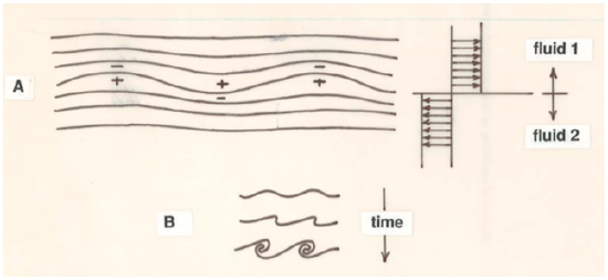
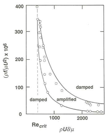
Figure \(\PageIndex{9}\) is a stability diagram for a laminar shear layer or boundary layer (see next section) developed next to a planar boundary. The diagram shows the results of both the mathematical stability analysis described above and experimental observations on stability. The experiments were made by causing a small metal band to vibrate next to the planar boundary at a known frequency and observing the resulting velocity fluctuations in the fluid. Agreement between theory and experiment is good but not perfect; if the experimental results were completely in agreement with the calculated curve, they would all fall on it. The diagram shows that there is a well-defined critical Reynolds number, \(\text{Re}_{crit}\), below which the laminar flow is always stable but above which there is a range of frequencies at any Reynolds number for which the disturbance is amplified, so that the laminar flow is potentially unstable and becomes turbulent provided that disturbances with frequencies in that range are present.

Figure \(\PageIndex{9}\): Diagram showing stability of a laminar shear layer (boundary layer) developed next to a planar boundary. The vertical axis is a dimensionless measure of the frequency \(f\) of the imposed small-amplitude disturbances. The horizontal axis is a Reynolds number based on the thickness \(\delta\) of the boundary layer and free-stream velocity at the outer edge of the boundary layer. The solid curve is the calculated curve for neutral stability (Lin, 1955); the points represent experimental determinations of neutral stability (Schubauer and Skramstad, 1947).