9.7.2: Tide-induced residual transport of (medium to) coarse sediment

In this paragraph, we explore the sediment flux averaged over the tide and analyse the conditions under which a net import or export of (medium to) coarse sediment in the basin will occur (for fine sediment an additional effect occurs that is treated in Sect. 9.7.3). A larger influx than outflux of sediment leads to a net landward directed sediment flux; as a result the basin will import sediment. Vice versa for basins exporting sediment.

In Ch. 5 we discussed in detail the mechanisms that contribute to a residual sediment transport, eithers landwards or seawards:

• The asymmetry of the horizontal tide (Sects. 5.7.4 and 5.7.5);
• Tide-averaged residual currents (Sect. 5.7.6) along the channels.

The residual flow along the channels may be composed of for instance contributions due to river flow and as compensation for Stokes’ drift. The secondary flow patterns as discussed in Sect. 5.7.6 have no direct impact on the import or export of sediment from the basin.

In the analysis below, we approximate the tide-averaged residual flow by a constant and depth-averaged residual tidal velocity \(u_0\) in the channel direction. We further assume that \(M2\) (semidiurnal, 12.42 h period) is the dominant tidal-current constituent and that all other constituents are of a lesser order of magnitude. Further, the residual flow velocity \(u_0\) is assumed to be small compared to the amplitude of the \(M2\) tidal current. These conditions are reasonably satisfied in most tidal basins in the Netherlands.

Coarse sediment was defined in Ch. 6 as having a diameter such that \(W_s/u_* > 1\), where \(w_s\) is the fall velocity and \(u_*\) is the shear velocity. Coarse sediment is thought to respond instantaneously to the flow velocity (or alternatively the bed shear stress). In terms of the flow velocity we can write for the bed-load transport (defined as volumetric transport excluding pores in \(m^3/s/m\)) in the case of small bottom slopes:

\[S \approx c|u^{n - 1}|u\label{eq9.7.2.1}\]

The coefficient \(n\) is thought to lie in the range 3 to 5. In this course we mostly propose \(n = 3\), consistent with the Bagnold formulation for bed load (Eq. 6.7.2.8) in the case of small bed slopes. Further \(c = 10^{-7}\ m^{2-n} s^{n-1}\) to \(10^{-4}\ m^{2-n}s^{n-1}\). In this transport formulation, initiation of motion is not taken into account. This would further enhance the effect of asymmetry.

For suspended load transport of medium to coarse, non-cohesive bottom material (sand) often a similar expression is used, but with a higher velocity power (\(n = 4\), in agreement with Bagnold’s suspended load formulation).

For suspended load transport of fine (cohesive) sediment other formulations need to be adopted, which take account of the time lags involved with settling and resuspension. This is treated in the Sect. 9.7.3.

The velocity signal considered by Van de Kreeke and Robaczewska (1993) can be written as:

\[u(t) = u_0 + \hat{u}_{M2} \cos (\omega_{M2} t) + \sum_{i} \hat{u}_i \cos (\omega_i t - \varphi_i)\label{eq9.7.2.2}\]

in which:

\(u_0\)	the Eulerian residual flow
\(\hat{u}_{M2}\)	the amplitude of the \(M2\) tidal current
\(\hat{u}_i\)	the amplitude of the other tidal current constituents
\(\omega_{M2}\)	the angular frequency of the \(M2\) constituent
\(\omega_i\)	the angular frequency of the other tidal current constituents
\(\varphi_i\)	the phase lag between \(M2\) and the other tidal constituents

By substituting this velocity signal (Eq. \(\ref{eq9.7.2.2}\)) in Eq. \(\ref{eq9.7.2.1}\), Van de Kreeke and Robaczewska (1993) demonstrated, under the assumption of \(M2\) dominance and \(n = 3\) (and thus \(S \propto u^3\)), what the most important contributions to net tide-induced bed load transport of coarse sediment are. Note that their approach is quite similar to the decomposition of the wave-induced cross-shore transport as discussed in Sect. 7.5.

The resulting expression for the long-term averaged bed load transport, valid under the above mentioned restrictions is:

\[\dfrac{S}{c \hat{u}_{M2}^3} = \underbrace{\dfrac{3}{2} \dfrac{u_0}{\hat{u}_{M2}}}_{1} + \underbrace{\dfrac{3}{4}\dfrac{\hat{u}_{M4}}{\hat{u}_{M2}} \cos \varphi _{M4-2}}_{2} + \underbrace{\dfrac{3}{2}\dfrac{\hat{u}_{M4}}{\hat{u}_{M2}} \dfrac{\hat{u}_{M6}}{\hat{u}_{M2}} \cos (\varphi _{M4-2} - \varphi _{M6-2})}_{3}\label{eq9.7.2.3}\]

in which:

\(u_0\)	the Eulerian residual flow
\(\hat{u}_{M2}\)	the amplitude of the \(M2\) tidal current
\(\hat{u}_{M4}\)	the amplitude of the \(M4\) tidal current
\(\hat{u}_{M6}\)	the amplitude of the \(M6\) tidal current
\(\varphi_{M4-2}\)	the phase lag between \(M2\) and \(M4\) (cf. Eq. 5.7.5.2)
\(\varphi_{M6-2}\)	the phase lag between \(M2\) and \(M4\)
\(c\)	coefficient defined through Eq. \(\ref{eq9.7.2.1}\)

Apparently, the long-term mean bed load transport is predominantly determined by:

• The residual flow velocity \(u_0\);
• The amplitude of the \(M2\) tidal current;
• The amplitudes and phases (relative to the \(M2\) tidal current) of the M4 (quarter-diurnal, 6.21 h period) and M6 tidal currents.

Although higher odd and even overtides also contribute, the first even overtide M4 and first odd overtide M6 are the most important contributing overtides. The components K1, S2, N2 and MS4 were also included in the analysis, but were found to only cause fluctuations of the transport rates that would average out in the longer term. For example, the effect of inclusion of S2 is only to give a beating of the transport flux with a period of about 14.7 days (cf. Fig. 3.25). The inclusion of the diurnal component merely gives a daily fluctuation but does not influence the longer term net transport (cf. Fig. 3.26).

The three numbered terms in the right-hand side (RHS) of Eq. \(\ref{eq9.7.2.3}\) represent the net transport as a result of:

1. The asymmetry introduced by the addition of a small residual flow to the sinusoidal M2 tidal current component (cf. Fig. 5.72 for a mean river discharge, although in that case \(u_0\) is not small);
2. The asymmetric velocity signal of the \(M2+M4\) tidal current combined.The tide-averaged velocity of the \(M2 + M4\) tidal current is zero. However, due to the non-linear response of the sediment transport to the velocity, larger (positive and negative) velocities get relatively more weight in contributing to the transport. The result is a net transport in ebb or flood direction respectively depending on the phase angle \(\varphi_{M4-2}\) (cf. Fig. 5.71); For \(\varphi_{M4-2} = \pi /2\) or \(3\pi /2\) the ebb and flood velocity are of the same size and the signal has a saw-tooth shape. The net transport (averaged over the tidal cycle) is zero. For other values of \(\varphi_{M4-2}\) the maximum ebb velocities differ from the maximum flood velocities (either larger or smaller in the case of ebb- or flood-dominance respectively), giving rise to a net sediment transport. The net transport is largest for the maximum skewness of the velocity signal (\(\varphi_{M4-2} = 0\) or \(\pi\));
3. An interaction term among \(M2\), \(M4\) and \(M6\) (smaller than the first two contributions). The importance of it is governed by the phase angles \(\varphi_{M4-2}\) and \(\varphi_{M6-2}\).

The first two terms in Eq. \(\ref{eq9.7.2.3}\) are the most important terms. Their origin can be further clarified by considering the effect of the addition to the \(M2\) sinusoidal current signal of \(u_0\) and the \(M4\) tidal current separately. We will also explore the effect of inclusion of \(M6\).

Let us first consider \(u(t) = u_0 + \hat{u}_{M2} \cos (\omega_{M2} t)\). If we substitute this in Eq. \(\ref{eq9.7.2.1}\) and use \(n = 3\), we find for the time-dependent transport:

\[\begin{array} {rcl} {S(t)} & \approx & {cu(t)^3 = c(u_0 + \hat{u}_{M2} \cos (\omega_{M2} t))^3 \Rightarrow} \\ {\dfrac{S}{c\hat{u}_{M2}^3}} & = & {\underbrace{\left (\dfrac{u_0}{\hat{u}_{M2}} \right )^3}_{1} +} \\ {} & \ & {\underbrace{3 \left (\dfrac{u_0}{\hat{u}_{M2}} \right )^2 \cos (\omega_{M2} t) + \cos^3 (\omega_{M2} t)}_{2} +} \\ {} & \ & {\underbrace{3 \left (\dfrac{u_0}{\hat{u}_{M2}} \right )^2 \cos^2 (\omega_{M2} t)}_{3}} \end{array}\]

The term denoted ‘1’ can be neglected relative to the other terms, since we had assumed that \(u_0 /\hat{u}_{M2}\) is a small quantity (\(M2\) being dominant). The remaining expression could also be obtained by using a Taylor expansion as in Intermezzo 7.3, now with the residual flow velocity being the perturbation. The terms denoted ‘2’ are symmetrical about the horizontal axis and will not give a contribution when averaged over the \(M2\) tidal period. The only term of interest for the tide-averaged sediment transport is term ‘3’. Integration over the tidal period results in:

\[\dfrac{\langle S \rangle}{c \hat{u}_{M2}^{3}} = \dfrac{3}{2} \left (\dfrac{u_0}{\hat{u}_{M2}} \right)\]

which is identical to the first term in Eq. \(\ref{eq9.7.2.3}\) and represents the effect of the interaction of a (small) residual flow and the \(M2\) tidal current.

Figure 9.28: \(M2\) and \(M4\) tidal current constituents. Flood dominance is found for \(-\pi/2 < \varphi_{M4-2} < \pi /2\) and ebb-dominance for \(\pi /2 < \varphi_{M4-2} < 3\pi /2\). Flow reversal from flood to ebb (high water slack) is of shorter duration than low water slack for \(0 < \varphi_{M4-2} < \pi\) and of longer duration for \(\pi < \varphi_{M4-2} < 2\pi\).

Figure 9.29: \(u\) and \(\langle u^3 \rangle\) for \(u\) consisting of \(M2\) and \(M4\) tidal current constituents with four different phase angles between \(M2\) and \(M4\). Since \(\langle S \rangle \propto \langle u^3 \rangle \) we find \(\langle S \rangle > 0\) for \(-\pi /2 < \varphi_{M4-2} < \pi /2\) and \(\langle S \rangle < 0\) for \(\pi /2 < \varphi_{M4-2} < 3\pi /2\). \(\langle S \rangle = 0\) for \(\varphi_{M4-2} = \pi /2\) and for \(\varphi_{M4-2} = 3/2\pi\).

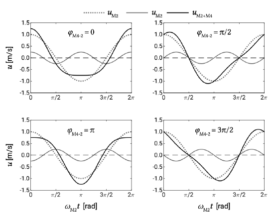
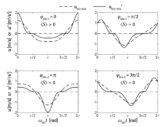
The next step is to look at the interaction of \(M2\) and \(M4\). The velocity can now be written as \(u(t) = \hat{u}_{M2} \cos (\omega_{M2} t) + \hat{u}_{M4} \cos (\omega_{M4} t - \varphi_{M4-2})\) with \(\omega_{M4} = 2 \omega_{M2}\). The phase lag \(\varphi_{M4-2}\) between \(M2\) and \(M4\) is \(\varphi_{M4} - 2 \varphi_{M2}\). The effects of the phase angle on the velocity signal and \(u^3\) are illustrated in Figs. 9.28 and 9.29.

We now get:

\[S(t) \approx c (\hat{u}_{M2} \cos (\omega_{M2} t) + \hat{u}_{M4} \cos (\omega_{M4} t - \varphi_{M4-2}))^3\label{eq9.7.2.6}\]

The tide-averaged transport can be obtained by integration of Eq. \(\ref{eq9.7.2.6}\). Analogous to the derivation of the \(M2\)-residual flow interaction, we neglect the third power of \(\hat{u}_{M4} /\hat{u}_{M2}\). This leads to:

\[\dfrac{\langle S \rangle}{c \hat{u}_{M2}^3} = \dfrac{3}{4} \left (\dfrac{\hat{u}_{M4}}{\hat{u}_{M2}} \right ) \cos \varphi_{M4-2}\]

In this expression we can recognise term ‘2’ Eq. \(\ref{eq9.7.2.3}\). It represents the effect of the interaction of the \(M2\) tidal current and its \(M4\) overtide. As mentioned already, for \(\cos \varphi_{M4-2} = \pm 1\) this interaction term is at its maximum. This corresponds to the situation that the ebb and flood velocities differ most in magnitude. In the case of \(\cos \varphi_{M4-2} = -1(\varphi_{M4-2} = \pi )\) the velocity signal is flood-dominant (see Fig. 9.28, top left) without any saw-tooth asymmetry, leading to a maximum net import of (coarse) sediment (Fig. 9.29, top left). For \(\cos \varphi_{M4-2} = -1\) (\(\varphi_{M4-2} = \pi\)) the velocity is ebb-dominant and the system exports sediment (see Figs. 9.28 and 9.29, bottom left). There is no contribution to the net sediment transport for \(\cos \varphi_{M4-2} = 0\) (\(\varphi_{M4-2} = \pi /2\) or \(3\pi /2\)), see the right panels of Figs. 9.28 and 9.29. This corresponds to a velocity signal that demonstrates saw-tooth asymmetry, but has equal flood and ebb current magnitudes and durations.

Figure 9.30: \(M2\) and \(M6\) tidal current constituents for four different phase angles between \(M2\) and \(M6\).

Figure 9.31: \(u\) and \(\langle u^3 \rangle\) for \(u\) consisting of \(M2\) and \(M6\) tidal current constituents with four different phase angles between \(M2\) and \(M6\). \(\langle S \rangle \propto \langle u^3 \rangle = 0\) for all phase angles.

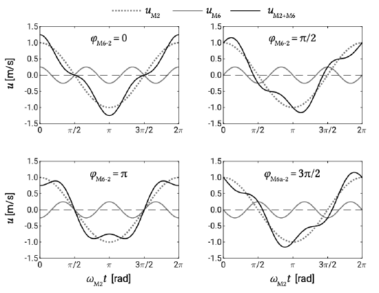
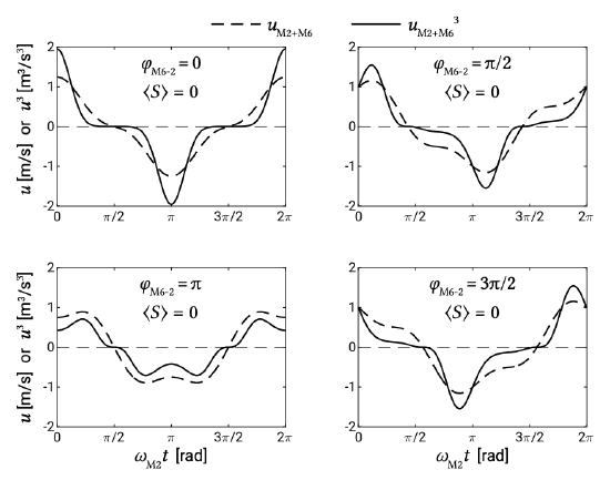
Why is a comparable term containing the odd overtide \(M6\) not visible in Eq. \(\ref{eq9.7.2.3}\)? Apparently the interaction between the \(M2\) and \(M6\) does not lead to a net sediment transport, regardless of the phase angle. The combination of \(M2\) and \(M6\) leads to saw-tooth asymmetry only (see Fig. 9.30), and therefore does not give a residual sediment transport (Fig. 9.31).

Combining the above with our knowledge about how the basin influences the tidal asymmetry, we may conclude:

Flood-dominant systems (with shallow channels and limited intertidal storage) enhance landward near-bed transport and tend to fill in their channels with coarse material, whereas ebb-dominant systems (with deep channels and large intertidal storage) enhance seaward near-bed transport and flush coarse sediment seaward.