8.3.2: Single Line Theory

Beach profile schematization

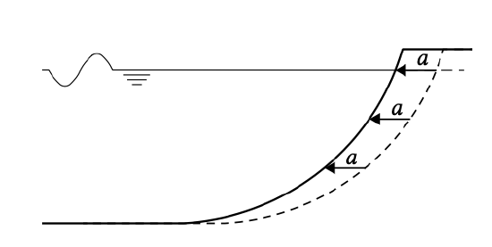
The basic assumption is that the shape of the cross-shore profile does not change in time, which implies an equilibrium profile of arbitrary shape. As the coast erodes or accretes, the entire profile moves seaward or landward with a horizontal distance \(a\). Figure 8.7 shows that this assumption requires also the assumption of a more or less horizontal part in the underwater profile; otherwise, unrealistic large quantities of sand are required for a small seaward movement of the shoreline.

Figure 8.7: Beach profile schematization in single line or one-line theory.

In practical applications, the closure depth (see Sects. 1.5.1 and 7.2.3 is taken as the lower limit of the coastal profile. Depth changes seaward of this closure depth are assumed to not directly contribute to the shoreline dynamics. The closure depth is governed by the highest waves that may occur in a certain period of time (normally several years). For the Holland coast (the central Dutch coast) the order of magnitude of the closure depth is MSL−6 m to MSL−12 m.

The upper limit of the coastal profile that needs to be taken into account depends – on shorter timescales – on whether the coast is eroding or not. For an eroding coast, the upper limit should be the dune height, allowing volume changes of the dunes. In the case of accretion, the upper limit is determined by the representative wave run-up added to the high water level. (It is thus assumed that the build up of the dunes by aeolian transport is a very slow process). This is usually about \(1\ m\) to \(3\ m\) above MSL. In the discussions below, we simply assume that the active profile has a height \(d\).

The wave characteristics in the assumed horizontal part are needed to compute changes in the schematised beach. Note that these characteristics are not necessarily equal to the deep water characteristics.

Governing equations

Consider a stretch of a beach that is changing – either eroding or accreting. The \(x\)-axis is roughly parallel to the coastline, the \(y\)-axis is normal to the coast, see Fig. 8.8. The position of the coastline is at \(y = Y\).

Figure 8.8: Longshore transport \(S_x\) and coastal change \(\Delta Y\) in a coastline model.

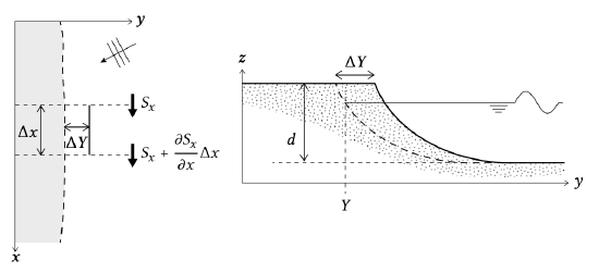
If during a short time interval \(\Delta t\) the shoreline moves forward with \(\Delta Y\), the amount of accumulated volume, over a distance \(\Delta x\) is:

\[\Delta x \Delta Y d\]

The net volume of sediment entering the segment with length \(\Delta x\) during time \(\Delta t\) is:

\[-\dfrac{\partial S}{\partial x} \Delta x \Delta t\]

Equating the accumulation of sediment and the net inflow of sediment yields the following continuity equation:

\[\dfrac{\partial Y}{\partial t} + \dfrac{1}{d} \dfrac{\partial S_x}{\partial x} = 0\label{eq8.3.2.3}\]

In Sect. 8.2.3 we had seen that the angle of wave attack relative to the coastline is an important variable in determining the sediment transport \(S_x\). Via the chain rule we can therefore write Eq. \(\ref{eq8.3.2.3}\) as:

\[\dfrac{\partial Y}{\partial t} + \dfrac{1}{d} \dfrac{\partial S_x}{\partial x} \dfrac{\partial \varphi}{\partial x} = 0\label{eq8.3.2.4}\]

Figure 8.9: Shoreline position \(Y\) in original position and after some time. In this figure is the original angle of wave incidence. After the change in shoreline orientation this angle has been reduced with \(\partial Y/\partial x\).

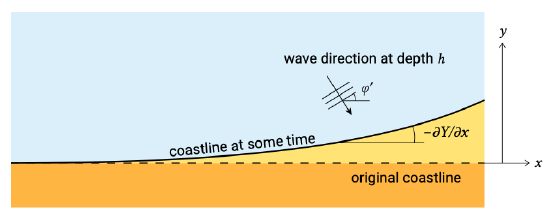
The term \(\partial S_x/\partial \varphi\) follows from any longshore transport formulation that we choose to use. In Sect. 8.3.3 we will do this analytically by assuming that the sediment transport formulation is a linear function of the angle of incidence. With a more complicated sediment transport formula, we can empirically determine \(\partial S_x /\partial \varphi\) by varying the angle slightly in the formula and calculating the transport rates. The term \(\partial \varphi /\partial x\) is directly related to the shoreline position that we are trying to solve for. This can be understood from Fig. 8.9 where an originally straight coastline is shown together with the coastline after some time.

The shoreline has rotated with an angle \(\partial Y/\partial x\). This directly implies a reduction of the angle of wave attack \(\varphi\) with \(\partial Y/\partial x\), since the wave angle is relative to the coastline. Hence, \(\varphi = \varphi' - \partial Y/ \partial x\) and \(\partial \varphi = - \partial Y/ \partial x\). Substituting this in Eq. \(\ref{eq8.3.2.4}\) gives:

\[\dfrac{\partial Y}{\partial t} - \dfrac{1}{d} \dfrac{\partial S_x}{\partial \varphi} \dfrac{\partial^2 Y}{\partial x^2} = 0\label{eq8.3.2.5}\]

Equation \(\ref{eq8.3.2.5}\) is a parabolic partial differential equation for the coastline position Y and must generally be solved numerically. It is the equation which is solved in coastline development models (such as Unibest-CL+ or Genesis, see Szmytkiewicz et al. (2000)). In this equation the angle \(\varphi\) is the angle of incidence at the closure depth.

In Sect. 8.2.4, the (\(S, \varphi\))-curve was introduced. We determined this curve by changing the angle of wave attack relative to a fixed coast. Since \(\varphi\) is the angle of wave attack relative to the coastline we could just as well have determined the curve by changing the coastline orientation relative to the waves, which is what we are doing in coastline modelling. The longshore sediment transport rate as a function of the changes in coastline orientation must be determined for the stretch of coast and the wave climate under consideration. This is done by calculating the longshore transport rates for the initial coastline orientation. Subsequently, the coastline orientation is changed a little bit and the longshore transport calculation is carried out again for the entire wave climate. This is equivalent to constructing a (\(S, \varphi\))-curve. An example of such a procedure is given in Intermezzo 8.2.

Intermezzo 8.2: Transport curve as computed in a coastline model

A transport curve in a coastline model describes the relation between the yearly averaged longshore transport \(S_x\) and the coastline orientation. To determine this curve, the full local wave climate needs to be taken into account, generally schematised as a limited set of individual conditions (see Sect. 8.2.5) that are each described by a number of parameters, namely:

• The significant wave height \(H_s\) (e.g. at the deep water boundary);
• The peak wave period \(T_p\);
• The angle of wave approach \(\varphi\) (e.g. at the deep water boundary);
• The storm-related set-up \(h_s\);
• The percentage of occurrence.

Each of the conditions contributes to the yearly-averaged transport weighted with their percentage of occurrence. The sum of the percentages of occurrence equals 100% (or 365 days per year, although one of the conditions may be a zero to small wave height).

Figure 8.10: Yearly-averaged transport as a function of changes in coastline orientation. The reference (initial) coastline orientation is \(0^{\circ}\).

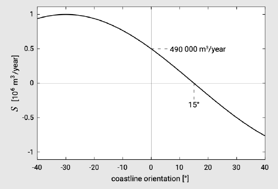
Figure 8.10 shows such a transport curve as computed with the coastline model Unibest-CL+ (https://www.deltares.nl/en/software/unibest-cl). For this computation a bottom slope of 1:100 was assumed from MSL to MSL−20 m. The sediment grain size \(D_{50} = 200\ \mu m\). The transport zone was assumed to extend to MSL−10 m. The wave input at MSL−20 m is given in Table 8.2 (wave angles are defined such that positive wave angles give positive sediment transports). A total of 16 wave conditions were defined in four wave height classes and four directional sectors. From the table it can be seen that the number of days per year with no waves to speak of is 365 - 181 = 184.

Table 8.2: Wave input: number of days of certain wave condition (combination of wave height and direction).

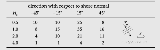
For the reference coastline orientation the yearly-averaged longshore transport is \(490\ 000\ m^3/yr\). If the coastline would rotate with \(15^{\circ}\), the total longshore transport becomes zero. The angle for which \(S = 0\) is sometimes called the equilibrium orientation, which is somewhat confusing since equilibrium requires zero gradients and not necessarily zero transports.

More insight in how to apply Unibest-CL+ can be obtained through e.g. Luijendijk et al. (2011) and Van der Salm (2013).

Note that the so-computed transport curve as a function of changing coastline orientation is not necessarily constant along the coast, for instance where local wave conditions are affected by wave sheltering. As an example, at either side of a shore-normal breakwater, waves from certain directions are affected by diffraction such that wave heights are reduced and the directions of the wave rays are more shore-normal. The alongshore variation of the yearly wave climate can be taken into account by relating a specific wave climate to a specific alongshore position and computing transport curves for various alongshore positions. In areas where the wave conditions are affected by non-uniform bottom topographies, by natural coastal features like headlands, or by man-made structures like breakwaters, it is important that the shape of the transport curve is allowed to change alongshore.