
8.2.3: Bulk longshore transport formulations
- Page ID
- 16383

The general transport formulations, which were compared in the previous section, were developed from the early seventies onwards (Bijker was the first to include the effect of waves in a general transport formulation, see Eq. 6.5.4.1). Before that time only bulk formulations were available. The bulk longshore transport formulation did not give the distribution over the surf zone, but only the total transport over the entire width of the littoral zone. Note however that, although the general formulations may resolve the cross-shore distribution over the surf zone, they are not necessarily better in predicting bulk transport rates, considering the large uncertainties involved in transport computations. Clear advantages of the bulk transport formulas are that they are robust and easy to calibrate and apply.
In this section, three bulk formulations are presented: 1) the Coastal Engineering Research Council (CERC) equation; 2) the formulation according to Kamphuis (1991); and 3) a formulation according to Bayram et al. (2007).
The CERC formula
Although one of the oldest longshore transport formulations, the CERC formula is still widely used. It has been developed by the Coastal Engineering Research Council (CERC) of the American Society of Civil Engineers (ASCE). The development of this formula took place in the late 1940s, well before longshore current theory was developed. The formula was calibrated using a large number of prototype and laboratory measurements.
The CERC formula gives the bulk longshore sediment transport – the total longshore sediment transport over the breaker zone – due to the action of waves approaching the coast at an angle. Hence, only the effect of the wave-generated longshore currents is included; tidal currents or other alongshore currents are not considered. If the longshore current is exclusively driven by waves, one can imagine that both the sediment concentration and longshore current velocity can be related in some way to the incident wave conditions. This is reflected in the CERC formula that reads in its most general form:
\[S = \dfrac{I}{\rho g(s - 1) (1 - p)} = \dfrac{K}{\rho g (s - 1)(1 - p)} (Enc)_b \cos \varphi_b \sin \varphi_b\label{eq8.2.3.1}\]
where:
| \(I\) | the immersed (underwater) weight of sediment transported, cf. Eq. 6.4.1.2 | \(N/s\) |
| \(S\) | the deposited volume of sediment transported | \(m^3/s\) |
| \(\rho\) | density of the water | \(kg /m^3\) |
| \(s\) | the relative density of the sediment \(\rho_s /\rho\) | - |
| \(p\) | porosity | - |
| \(g\) | gravitational acceleration | \(m/s^2\) |
| \(K\) | coefficient | - |
| \(E\) | wave energy | \(J/m^2\) |
| \(c\) | the wave phase velocity | \(m/s\) |
| \(n\) | the ratio between group and phase velocity | - |
| \(\varphi\) | the wave angle of incidence | - |
| \(b\) | subscript referring to conditions determined at the outer edge of the breaker zone | - |
Equation \(\ref{eq8.2.3.1}\) is a dimensionally correct form of the CERC formula as presented by Komar and Inman (1970). The original CERC formula had a dimensional coefficient (such that the coefficient was dependent on the units used) and was formulated in terms of US Customary Units. The Komar and Inman form does not have this problem.
According to Eq. \(\ref{eq8.2.3.1}\) the bulk longshore sediment transport rate \(S\) is a function of the product of the energy flux \((Enc)_b\) at the point of breaking (see also Eq. 5.2.2.1) and \(\cos \varphi_b \sin \varphi_b\). This term \(P = (Enc)_b \cos \varphi_b \sin \varphi_b\) was named ‘longshore component of wave power’ and its physical interpretation has been the topic of many discussions over the years. It was not until 1972 – years after the original presentation of the CERC value – that Longuet-Higgins related \(P\) to the then new concept of radiation stresses (Sect. 5.5.2). From Eq. 5.5.2.13 and Fig. 5.30 it becomes clear that \(P\) is the shear component of the radiation stress at the breaker point multiplied by \(c\) at the breaker point: \(P = S_{yx, b} c_b\). We know that the cross-shore gradient in radiation shear stress is responsible for driving the longshore current (Eq. 5.5.5.1). The radiation shear stress at the point of breaking can therefore be seen as this driving force integrated over the surf zone. But that still does not explain how the product of \(S_{yx, b}\) and \(c_b\) should be interpreted. The CERC formula was probably rather intuitively derived. Inman and Bagnold (1963) derived a bulk longshore transport formula in a more fundamental way, namely based on an energetics approach and found a formula similar in form to the CERC equation. This is demonstrated in Intermezzo 8.1.
Often the CERC equation is rewritten in terms of wave height parameters by substituting \(E = \dfrac{1}{8} \rho g H_b^2\). Shallow water wave breaking is assumed such that \(n_b\) can be taken equal to 1 and \(c \approx \sqrt{gh_b}\) in which \(h_b\) is replaced with \(H_b/\gamma\). For the breaker index often a value of 0.78 is assumed. (Sect. 5.2.5). Using the double angle formula \(2\cos \varphi_b \sin \varphi_b = \sin 2\varphi_b\), the CERC formulation Eq. \(\ref{eq8.2.3.1}\) can be expressed as:
\[S = \dfrac{K}{16(s - 1)(1 - p)} \sqrt{\dfrac{g}{\gamma}} \sin 2 \varphi_b H_b^{2.5}\label{eq8.2.3.2}\]
For irregular waves, the value of the coefficient \(K\) depends on whether for the wave height at breaking \(H_b\) the root mean square wave height \(H_{rms}\) or the significant wave height \(H_s\) is used. A value of \(K\) for \(H_{rms} = 0.77\) was derived from a field study by Komar and Inman (1970) corresponding to \(H_{rms}\). This is the value that is commonly seen in many longshore transport rate computations. In the Shore Protection Manual, the US Army Corps of Engineers mentions a value of \(K_{\text{for} H_{rms}} = 0.92\). In more recent studies, Schoonees and Theron (1993, 1996) suggested a significantly lower value of the coefficient, namely about half, based on a re-examination of available field data. For a specific project, it is best to determine the coefficient by calibration. Engineers often prefer to use for \(H_b\) the significant wave height \(H_s\) at breaking. In that case the value of the coefficient \(K_{\text{for} H_{s}}\) is smaller, viz. \(K_{\text{for} H_{s}} = \left (\dfrac{1}{\sqrt{2}} \right )^{5/2} K_{\text{for} H_{rms}} \approx 0.4 K_{\text{for} H_{rms}}\) (since for a Rayleigh distribution: \(H_s = \sqrt{2} H_{rms}\), see Table 3.1).
Inman and Bagnold (1963) applied the energetics concept of Bagnold (1963), as explained in Sect. 6.7.2, to the littoral zone. In the surf zone, the wave oscillatory motion, with angle of incidence \(\varphi\), is thought to set an amount of sediment into motion without resulting in a net transport. The sediment supported by the wave action (with a total immersed weight \(W\)) is passively advected with a representative longshore current velocity \(V\), such that the bulk immersed weight longshore transport rate is given by \(I = WV\).
Per unit crest width, the wave power (rate of transport of energy) that is available for dissipation in the entire surf zone is equal to \((Ec_g)_b\), see Eq. 5.2.1.3, with \(b\) referring to the values at the breaker line. The crucial assumption now is that a proportion \(\varepsilon\) of the wave power is dissipated by means of bottom friction and used in transporting sediment as bed load. The mean frictional force applied to the whole of the sediment bed per unit crest width is proportional to \((Ec_g)_b /\hat{u}_b\) where \(\hat{u}_b\) is mean frictional velocity relative to the bed within the surf zone and is assumed to be proportional to the orbital velocity near the bottom just before wave breaking. Per unit shoreline the frictional force is proportional to \((Ec_g)_b \cos \varphi_b /\hat{u}_b\).
The frictional resistance of the sediment is equal to \(\mu W\), in which the friction coefficient \(\mu = \tan \varphi_r\) is the tangent of the internal angle of repose indicated by \(\varphi_r\). Equating the frictional force on the bed and the resisting force leads to \(W = \varepsilon (Ec_g)_b \cos \varphi_b /(\mu \hat{u}_b)\). Hence, according to Inman and Bagnold:
\[I = WV = \varepsilon \times \dfrac{(Ec_g)_b \cos \varphi_b}{\mu \hat{u}_b} V \label{eq8.2.3.3}\]
Let us now rewrite the analytical result for the longshore current velocity (Eqs. 5.5.5.11 and 5.5.5.12) using the shallow water approximation Eq. 5.4.1.2 for the orbital velocity. This gives for the maximum longshore current velocity at the breaker line (a representative longshore current velocity \(V\) at a mid-surf zone location would have half of this maximum value):
\[V_b = \dfrac{5}{8} \pi \dfrac{\tan \beta}{c_f} \hat{u}_b \sin \varphi_b \label{eq8.2.3.4}\]
Substitution in Eq. \(\ref{eq8.2.3.3}\) yields:
\[I = \text{constant} \times \dfrac{\tan \beta}{c_f \mu} (Enc)_b \cos \varphi_b \sin \varphi_b \label{eq8.2.3.5}\]
Neglecting dependencies on the beach slope and the physical properties of the sand yields:
\[I = \text{constant} \times (Enc)_b \cos \varphi_b \sin \varphi_b\]
This is identical in form to the CERC equation Eq. \(\ref{eq8.2.3.1}\). We have however not been totally consistent, since in the derivation of Eq. \(\ref{eq8.2.3.4}\) we assumed
Equation \(\ref{eq8.2.3.2}\) is a very practical form of the CERC equation. It shows that, as long as the other parameters are constant, the transport magnitude increases with increasing wave angle at the breaker point until a maximum is reached at \(\varphi_b = \pm 45^{\circ}\) (in practice will be in the range \(-20^{\circ}\) to \(20^{\circ}\) due to refraction). Interesting is also that the longshore transport is proportional to the wave height to the power of 2.5. This can be interpreted, using Intermezzo 8.1, as a sediment load proportional to \(E_b\) and hence to \(H_b^2\) that is transported with a velocity proportional to \(\hat{u} = \dfrac{1}{2} \sqrt{g \gamma H_b}\) and hence to \(\sqrt{H_b}\). The breaking parameter is often taken as a constant (0.78). However, from Sect. 5.2.5 it is known that the breaking parameter increases with increasing Iribarren parameter (Eq. 5.2.5.5), hence with increasing relative steepness of the slope. A larger relative bottom slope (larger bottom slope or longer wave) would therefore slightly decrease the sediment transport, at least according to the CERC formula. This is however only a weak dependence in the CERC equation, and for all practical purposes one may consider the formula to be independent of wave period or bottom slope.
In some applications it is more practical to use deep water wave parameters in the equations. The conversion to deep water parameters is quite straightforward, when using an important finding of Sect. 5.5.5. There it was explained that if the water depth contours in the area are all parallel, \(S_{yx}\) does not vary outside the breaker zone. Hence: \(P = S_{yx, b} c_b = S_{yx, 0} c_b\). We can thus evaluate \(S_{yx}\) using deep water wave characteristics, which means that all wave parameters can thus be taken as deep water parameters except for \(c_b\). Remember that in deep water we need to take \(n_0 = \dfrac{1}{2}\). This yields for straight parallel depth contours:
\[S = \dfrac{K}{32(s - 1)(1 - p)} c_b \sin 2 \varphi_0 H_0^2\]
There are many equivalent forms of the CERC equation and all of them have at least one wave parameter at the breaker line. Due to the different representations, any application of the CERC formula must be made carefully (like of course with all types of sediment transport formulas). This holds in particular for the value of the coefficient, the choice of \(H_{rms}\) or \(H_s\) and the choice for deep water wave parameters or parameters at the breaker line.
Limitations of the CERC formula
Due to its simplicity the CERC formula can be helpful in understanding and solving many practical problems. The following prices have been paid to achieve the simplicity of the CERC formulation (some of which have already been mentioned):
- The first limitation is that only the wave-induced longshore current is taken into account; all other alongshore current driving forces, such as tidal currents, are ignored. In order to take the latter into account more general transport formulations need to be applied. In a formulation of the form Eq. \(\ref{eq8.2.3.3}\), in principle, also tidal and wind-driven alongshore currents could be used;
- The second limitation is that the sand transport is independent of the sand properties such as grain size. Also, the beach slope and hence the type of breakers is ignored (although the breaker index may be assumed to be dependent on the breaker type). Eq. \(\ref{eq8.2.3.5}\) already suggested a dependency on beach slope and grain properties. To include these variables the formulation of Kamphuis (below) can be used;
- A third limitation is that only the total sediment transport in the breaker zone is given. It is often of practical importance to know how this transport is distributed over the width of the breaker zone, for instance if bars are present in the coastal profile, or if coastal structures are considered that do not entirely cover the breaker zone (such as groynes: see Ch. 10). However, this distribution could be estimated from a distribution for the longshore current velocity and wave stirring capacity.
Grain size and beach slope
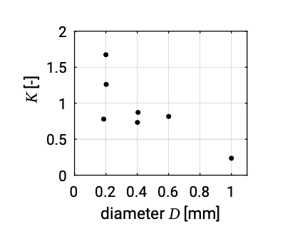
Dean et al. (1982) suggested that the coefficient \(K\) in Eq. \(\ref{eq8.2.3.2}\) should be dependent on the grain size, see Fig. 8.3.
Such a relation is not unexpected since the CERC formula only has the wave characteristics and one can expect the sediment transport to depend on the sediment properties too, with larger transport for smaller grain sizes. It is often believed that the transport should be inversely proportional to the grain size to a power of about three, hence \(S = f(D^{-3})\). The CERC formula was originally derived for beaches with uniform sand ranging between \(175\ m\) to \(1000\ m\) and thus represents an average over this range of conditions.
Kamphuis (1991) made an analysis of field and lab data and suggested an alternative bulk longshore transport formulation that includes the effects of not only grain size but beach slope and wave steepness as well.
His formulation for the immersed mass of transported sediment \(I_m = \rho (s - 1)(1 - p)S\) (see Eq. 6.4.1.2):
\[I_m = 2.27 H_{s, b}^2 T_p^{1.5} (\tan \alpha_b)^{0.75} D^{-0.25} (\sin 2\varphi_b)^{0.6} \label{eq8.2.3.8}\]
with \(\tan \alpha_b\) is the beach slope at the breaker point.
The wave period, grain size and beach slope (absent in the CERC equations) now influence the longshore transport rate. Note that the dependency on the wave angle seems relatively weak as compared to the CERC formulation. Also the grain-size proportionality with \(D^{-0.25}\) seems to be rather weak. However, it should be realised that the variables in the empirically derived Eq. \(\ref{eq8.2.3.8}\) are interdependent. For example: given constant hydraulic conditions, coarser beach materials tend to form steeper slopes1; gravel beaches are far steeper than sand beaches. On the other hand, if the beach material is of a given diameter, then higher waves tend to result in flatter beach slopes. Similarly, the wave parameters \(T_p\), \(\varphi_b\) and \(H_{s, b}\) are interrelated.
Recent bulk longshore transport formulation
Bayram et al. (2007) presented a new bulk formula based on the energetics concept, similar to Inman and Bagnold’s model in Intermezzo 8.1. By assuming that the dissipated fluid power maintaining the sediment load is dissipated by bottom friction, Inman and Bagnold considered sediment transported as bed load. By contrast, Bayram et al. assume that suspended sediment transport is the dominant mode of transport in the surf zone, as a result of turbulence induced by breaking waves. They assume that the dissipated fluid power per unit shore length used in suspending sediment is \(\varepsilon (Ec_g)_b \cos \varphi_b\) (similar to Intermezzo 8.1). The difference now is that the work done (per unit time) in maintaining the suspended load at a certain level is the product of \(W\) times the fall velocity \(w_s\). Hence: \(W = \varepsilon (Ec_g)_b \cos \varphi_b /w_s\).
Instead of Eq. \(\ref{eq8.2.3.3}\) we now get:
\[I = WV = \dfrac{\varepsilon (Ec_g)_b \cos \varphi_b}{w_s}V\]
For \(V\) an analytical solution is used for the mean longshore current velocity that is derived using a Bruun-Dean’s equilibrium profile (Eq. 7.2.2.1) instead of a constant bed slope. Based on comparison with field and laboratory data, Bayram et al. (2007) conclude that the predictive capability of their formula is higher than of the CERC, Inman-Bagnold and Kamphuis formulas. A recent attempt to improve the accuracies of these bulk longshore transport formulas is Mil-Homens et al. (2013).
1. Kamphuis (2000) mentions this as the probable reason for the absence of the grain-size and beach slope dependency in the CERC formula. In addition, for grain sizes in the order of \(200\ \mu m\) the grain-size dependency is not so clear according to Fig. 8.3.