7.2.1: The concept

Figure 7.5: Upper shoreface profile variation for Ameland (upper panel), Egmond (middle panel) and Noordwijk (lower panel) over the period 1965–2019. The cross-shore distance is relative to the a local beach pole or Rijksstrandpaal (RSP) in Dutch. The average HW and LW lines are also indicated. Note the significantly stronger variability of Ameland’s dune and nearshore profile as compared to the other two locations. (Data from JARKUS, n.d.).

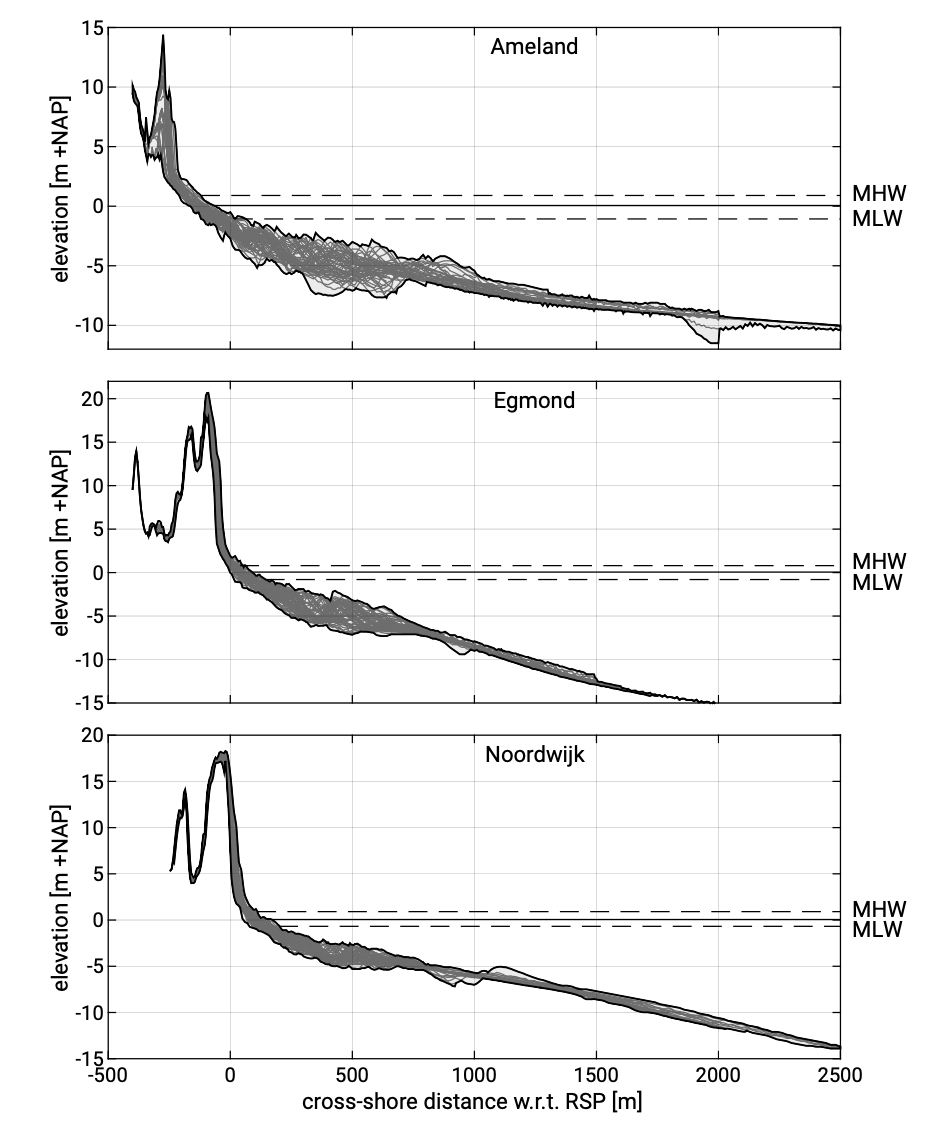
Consider a coastal stretch that has no alongshore sediment transport gradients. If we then adopt the coastal engineering assumption that the amount of sediment in the upper shoreface remains constant, the shoreline position will remain the same when averaged over several years. Figure 7.5 shows the Ameland, Egmond and Noordwijk shoreface profiles (Fig. 7.3) from 1965–2019 (from the JARKUS (n.d.) database with yearly measurements along the Dutch coast). The cross-shore distance is relative to a local beach pole or Rijksstrandpaal (RSP) in Dutch. In order to cancel any structural gains or losses, the profiles have been shifted to the same duneface location (Fig. 7.6).

Figure 7.6: Upper shoreface profile variation for Ameland (upper panel), Egmond (middle panel) and Noordwijk (lower panel) over the period 1965–2019. The profiles have been shifted to the same duneface location (MSL +3 m), so any structural gains or losses are cancelled. The average HW and LW lines are also indicated. (Data from JARKUS, n.d.).

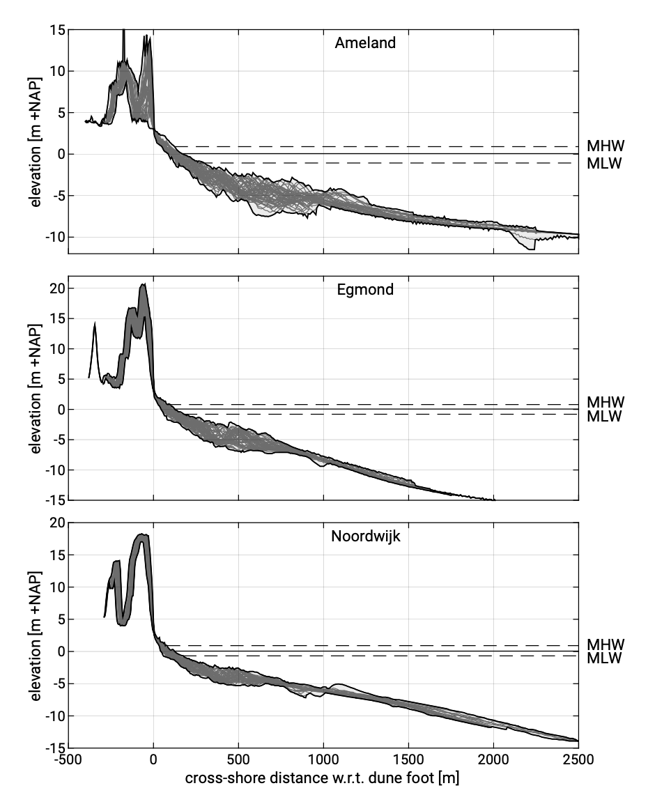
We observe that the various profiles show a dynamic variation that is clearly related to the position of the bar(s). We will discuss bars further on. What we also observe is that the profile variations remain in an envelope that seems stable over the years. One may therefore speak of the existence of a dynamic equilibrium profile (e.g. as follows from a best fit through the profile data).

It is commonly assumed that if one exposes, e.g. in the laboratory, a beach profile to constant wave forcing at a fixed water level, a stable equilibrium profile (cross-shore profile of constant shape) will be reached after a sufficiently long time. Is there a relation between this stable equilibrium profile and the dynamic equilibrium profile as found in the field? The answer is partly yes and partly no. We may expect that also a shore profile in the field will respond to a constant forcing condition and that it will search for an equilibrium form to that forcing. However, in nature the forcing (waves and water levels) is far from constant and varies so rapidly that a stable equilibrium is never reached. It is for this reason that the shoreface profile continuously oscillates in response to the varying forcing. However, interestingly enough these oscillations are confined to a steady envelope, the mean position of which we define as a dynamic equilibrium profile.

In the following sections we will first describe empirical and semi-empirical approaches to generalise the best profile fit for arbitrary upper shoreface profiles (Sect. 7.2.2). Second, in Sect. 7.2.3, we will discuss the engineering applications of the dynamic equilibrium concept.