6.5.4: Bed load transport based on time-averaged shear stress

Considerably simpler are the bed load formulations in which instead of the instantaneous bed shear stress, the time-averaged bed shear stress is used. Bijker (1967) was the first to present such a model (of the form of Eq. 6.5.2.5) for the combination of waves and currents. As a starting point he used the Kalinske-Frijlink bed load transport formulation for currents only. This empirical formulation had been used extensively for river applications. Bijker adjusted this formulation for the combined-wave current situation, by assuming that the effect of waves is to enhance the stirring of sediment which is consequently transported by the mean current. Later we will explain in some detail that this assumption is especially valid for longshore sediment transport calculations (oscillatory movement approximately perpendicular to the current). The Bijker formulation 1967 is given here as an example of a transport formulation for time-averaged bed load transport:

\[S_b = BD_{50} \underbrace{\dfrac{U}{C}\sqrt{g}}_{\text{current only transports the sediment}} \exp \underbrace{\left [\dfrac{-0.27(s - 1) D_{50} \rho g}{\mu \langle |\tau_{cw} | \rangle} \right ]}_{\text{wave-current shear stress stirs up the sediment}} \label{eq6.5.4.1}\]

where:

\(B\)	Bijker coeefficient (= 5)	-
\(D_{50}\)	representative particle diameter	\(m\)
\(U\)	current velocity (e.g. longshore current)	\(m/s\)
\(s\)	relative density \(\rho_s /\rho\)	-
\(C\)	Chezy coefficient (see Intermezzo 5.2)	\(m^{1/2}/s\)
\(\mu\)	ripple coefficient: part of the total bed shear that is available for transporting material	-
\(\langle | \tau_{cw}| \rangle\)	time-averaged shear stress magnitude for the combined wave-current motion	\(N/m^2\)

The value for the Bijker coefficient \(B\) has received much discussion. It has been suggested that the value of \(B\) should vary from 2 well outside the breaker zone to 5 inside the breaker zone. The main difference with the original Kalinske and Frijlink formula is the use of the time-averaged wave-current shear stress magnitude \(\langle |\tau_{cw}| \rangle\) instead of the time-averaged current-only bed shear stress. We can interpret Eq. \(\ref{eq6.5.4.1}\) as the product of the transporting mean velocity times the sediment load stirred up by the combination of waves and currents: \(S = U \times\) ‘sediment load’. In shallow water the contribution of the wave motion to the bed shear stress magnitude (and therefore to the stirring of sediment) is often more important than the contribution by the mean current. Therefore, it is often said that waves stir up the sediment, while currents transport it.

Bijker reasoned that at every moment in time, the bed shear magnitude determines the stirring of sediment, irrespective of the direction of this shear stress. Therefore, the bed load transport is dependent on \(\langle |\tau_{cw}| \rangle\) instead of on for instance the time-averaged bed shear stress \(\langle \tau_{cw} \rangle\). The difference between the two can be realised when considering a sinusoidal wave only, for which the bed shear oscillates symmetrically as well. The time-mean bed shear stress \(\langle \tau_{cw} \rangle\) is zero. Nevertheless, the waves are able to stir up sediment when the absolute value of the bed shear \(|\tau_{cw}|\) is larger than zero (no threshold of motion criterion is considered). Similarly, for the combination of waves and currents, the sediment load is determined by the shear stress magnitudes.

Figure 6.14: Left: plan view of velocity components \(u_t\) and \(V_t\) at a certain elevation \(z_t\) above the bed. Top right: the resultant velocity is \(V_r\) and varies in magnitude and direction during the wave cycle (between \(V_{r,\min}\) and \(V_{r,\max}\)). Bottom right: bed shear stress components during the wave cycle. Since \(\tau_{cw} \propto |V_r| V_r\) the larger velocities contribute relatively more to the bed shear stress.

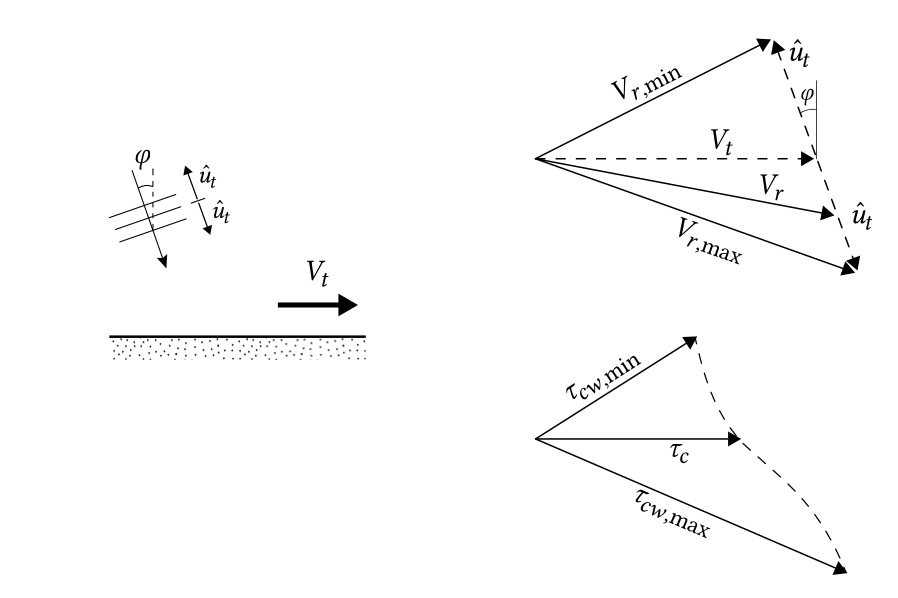
Bijker developed generalised formulations for the bed shear stress \(\tau_{cw}\) for waves at an arbitrary angle with the current. In Sect. 5.5.5 we had already seen that we cannot simply add up the shear stress due to currents and waves; due to the non-linear relationship between velocity and shear stress, we need to add the velocities instead (see Fig. 6.14).

Bijker started with a time-series of (linear) waves plus current at a certain height \(z_t\) above the bed, from which he derived – using an analytical turbulence model – approximate expressions for not only the mean bed shear stress in the direction of the current \(\tau_m\) but also for the mean shear stress magnitude \(\langle |\tau_{cw}| \rangle\). Bijker’s expression for the mean value of the bed shear stress magnitude under combined waves and currents reads:

\[\langle |\tau_{cw}| \rangle = \tau_c \left [1 + \dfrac{1}{2} \left \{\xi \dfrac{\hat{u}_0}{U} \right \}^2 \right ] \]

where

\(\hat{u}_0\)	maximum orbital velocity at top of wave boundary layer	\(m/s\)
\(U\)	depth-averaged velocity	\(m/s\)
\(\xi\)	combination of various parameters \(\xi = \sqrt{\dfrac{1}{2} \dfrac{f_w}{f_c}} = C \sqrt{\dfrac{f_w}{2g}}\)	-

This expression is dependent on the waves-only friction factor \(f_w\) (Eq. 5.4.3.7 and 5.4.3.8) and the current-only friction factor \(f_c\) (Eq. 5.4.3.6). It represents the average length of the vector \(\langle | \tau_{cw} | \rangle \) of Fig. 6.14 and is independent of the angle between waves and current.

For a typical surf zone situation with approximately normally incident waves (perpendicular to the longshore current velocity \(V\)) and under the assumption of \(\xi \dfrac{\hat{u}_0}{V} \gg 1\).

Bijker’s expression for the mean bed shear stress \(\tau_m\) in the current direction reduces to an expression identical to Eq. 5.5.5.6.

Bijker’s model for the wave-current shear stress is just one of many wave-current interaction models that can be used in morphodynamic models. Soulsby et al. (1993) compared various wave-current interaction models, ranging from the Bijker formulation to sophisticated wave boundary layer models and analysed how waves and currents in a combined wave-current motion contribute to the bed shear stress (see Intermezzo 6.3).

Intermezzo 6.3 Parameterisation of wave-current interaction models

Figure 6.12: Schematic for bed shear-stresses with wave-current interaction. (left) the current-alone stress (\(\tau_c\)), and (middle) the wave-alone stress (amplitude = \(\tau_w\)), combine non-linearly to give (right) stresses having mean \(\tau_m\) and maximum \(\tau_{\max}\). After Soulsby et al. (1993). The orbital velocity makes an angle \(\gamma\) with the mean current.

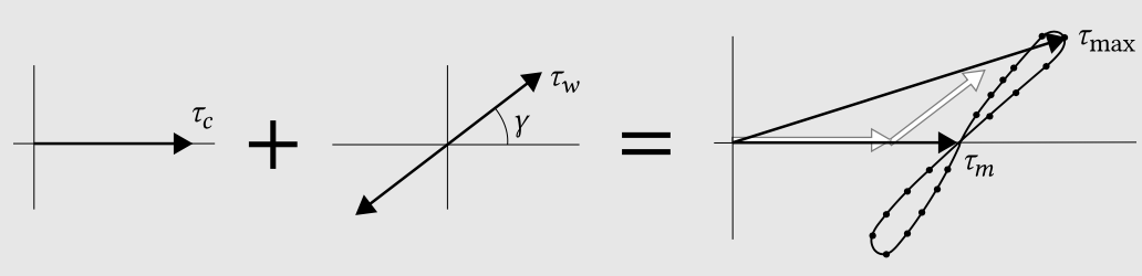
The two parameters that were considered in the intercomparison were the time-averaged bed shear stress in the direction of the current (denoted \(\tau_m\)) and the maximum bed shear stress (denoted \(\tau_{\max}\)). See also Fig. 6.12. The choice for these parameters is based on the fact that \(\tau_m\) is generally required for the computation of the mean current profile in wave-current motion, whereas the parameter \(\tau_{\max}\) is important to determine the threshold of motion and the entrainment of sediment. Both the maximum shear stress during a wave cycle and the mean shear stress in the current direction, were related to shear stresses that would occur if the wave and current only shear stresses could be summed linearly.

Figure 6.13: Intercomparison of various wave-current interaction models for an angle \(\gamma\) of \(0^{\circ}\) between waves and currents and for given values of \(z_0/h\) and \(\hat{\xi}_0/z_0\) where \(\hat{\xi}_0 = \hat{u}_0/\omega\) is the particle excursion amplitude (see Eq. 5.4.1.3) close to the bed and \(z_0 = k_s/30\) with \(k_s\) is the Nikuradse roughness height. Adapted from Soulsby et al. (1993).

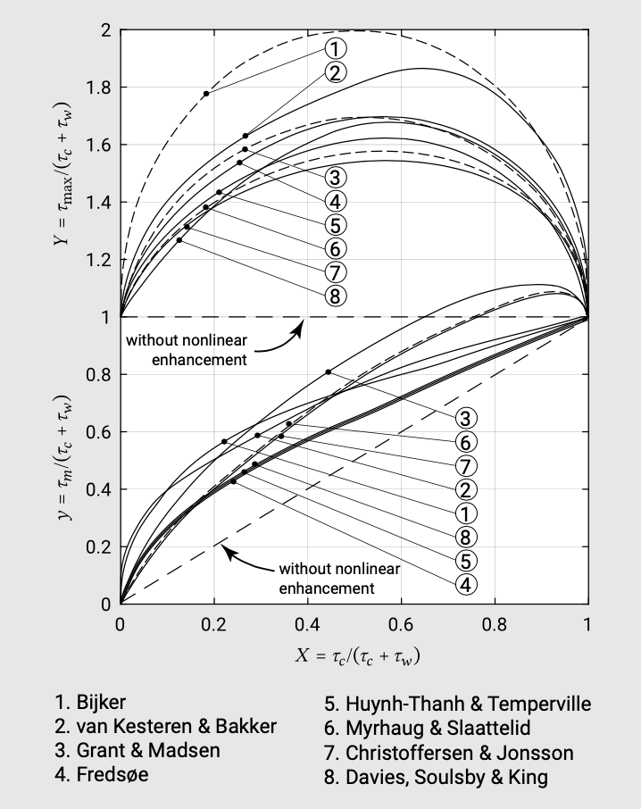
Figure 6.13 shows a result of this intercomparison. The lower figure shows that mean bed shear stress goes to zero for waves only and to the current only shear stress for currents only. For the combination of waves and currents, all models show the expected non-linear enhancement of the bed-shear stress when currents and waves are combined; the dotted line in both the upper and lower figure shows the result for a linear addition of the effect of waves and current (shear stress due to waves and currents simply added up). The models differ in the relative effect of waves and currents, with the Bijker model overestimating the effect of waves. This is related to the fact that the Bijker model does not take into account that the mean flow near the bed is reduced (and the shear stress enlarged) due to the extra resistance introduced by the wave boundary layer. In Fig. 6.12 it was already demonstrated that the angle between waves and current is important. Soulsby et al. (1993) showed that the non-linear enhancement decreased for angles \(\gamma\) going from \(0^{\circ}\) (waves and current aligned) to \(90^{\circ}\) (waves and current perpendicular).

The majority of the compared models require extensive computations for the prediction of the time-averaged bed shear stress. Soulsby et al. (1993) parameterised the models, so that they can be used in a computationally efficient way in morpho-dynamic models. The models are derived for monochromatic waves (a single harmonic). When applying the models to irregular waves, the orbital excursion amplitude should be based on the \(H_{rms}\) (the root-mean-square wave height, Sect. 3.4.2).