
3.5.2: Wave Dispersion
- Page ID
- 16294

In principle the wave motion can be described by the continuity equation and the Navier-Stokes equations of motion. Difficulties arise however when attempts are undertaken to solve these equations. One of the complications is that the surface boundary condition is the surface elevation that we try to solve. If we linearise this surface boundary condition and assume a horizontal bottom a simple solution to the equations is the single Fourier component that we described in Sect. 3.2. We then get the Airy wave theory (App. A). Neglecting non-linearities can be seen to be a good approximation for not too steep waves in deep water (\(ak \ll 1\) for \(kh\) is large) or small amplitude waves in shallow water (\(a \ll h\) for \(kh\) is small). According to Airy wave theory for a linear sine wave the relation between frequency \(\omega\) and wavenumber \(k\) is given by:
\[\omega = \sqrt{gk \tanh kh}\]
and is called dispersion relation. It is a function of the local water depth and the restoring force \(g\). The phase velocity \(c = \omega /k\) is then given by:
\[c = \dfrac{gT}{2\pi} \tanh kh = c_0 \tanh kh\]
The phase velocity (speed) is the rate at which any phase of the wave (for instance the wave crest) propagates in space. It is also called propagation velocity (or speed) or wave celerity. The nature of the hyperbolic tangent is shown in Fig. 3.10.
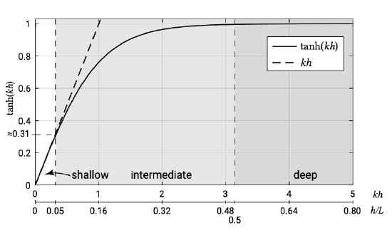
Given the fact that tanh \(kh\) equals 1 for \(kh \gg 1\), \(c_0\) represents the deep water phase velocity \(c_0 \approx 1.56T\) as function of \(T\). The deep water (or short wave) approximation can be used without too many errors (order of 1 %) for \(kh > \pi\) or \(h/L > 0.5\). Wind waves in oceanic waters can be considered as short waves, such that their phase velocity is linearly dependent on the wave period. Expressed in terms of the wavenumber in deep water the phase velocity \(c_0 = \sqrt{gL_0 /2\pi}\) and is therefore proportional to the square root of the deep water wavelength. Hence, longer waves propagate faster than shorter waves. Independent harmonic components of a wind wave field can be expected to travel at different speeds. The separation of the different harmonic components due to their different propagation speeds is called frequency dispersion. Oceanic wind waves are highly dispersive.
Since \(\tanh kh\) equals \(kh\) for \(kh \to 0\), the dispersion relation reduces to \(c = \sqrt{gh}\) for \(kh \to 0\). Hence, if the wave is long enough (\(kh < 0.31\) or \(h/L < 1/20\)), the wave celerity is only dependent on the local water depth. The shallower the water depth, the smaller the propagation speed is. Since the wave celerity is independent of the wave period the wave is called non-dispersive. This is the case for the tide and generally for tsunami waves as well. Wavelengths of tsunamis are easily \(100\ km\) or more2 which is more than 20 times larger than the average water depth in the deep ocean which is about \(4000\ m\) deep. A tsunami then propagates at a velocity of \(c = \sqrt{9.81 \times 4000} = 200\ m/s\) or \(700\ km/h\). As long as they do not dissipate their energy against a shore, tsunamis can travel at these high speeds for a long period of time and lose very little energy in the process.
If the waves meet a current (in or against the wave propagation direction), the wavelength, propagation velocity and wave height will be affected. The propagation velocity and wavelength relative to a fixed reference frame will increase in the case of a current in the propagation direction. The wave height will decrease. In the case of an opposing current it is the other way around.
2. In Sect. 3.2, tsunami periods were said to range from 5 min to 60 min. As an exercise: use Table A.3 to compute the corresponding wavelengths at a depth of 4000 m. Also compute the wave period range for which this depth is classified as intermediate water.