3.2: Oscillations of the ocean water surface

We can broadly define ocean waves as all sea-surface variations on the timescale of seconds to months as generated in the oceans. MSL is the sea level you get if you average these fluctuations out. This definition of ocean waves includes wind waves, tides and tsunamis. Wind and atmospheric pressure changes can also cause water level variations.

Figure 3.1: Simple representation of a wave. Left: the spatial variation is measured along the direction of wave propagation at a single moment in time. Right: the temporal variation in water level \(\eta\) is measured over a certain time period at a single location (at location 2 and directly following the recording of the spatial variation). A similar signal measured simultaneously at location 1 (or 3) will have opposite sign.

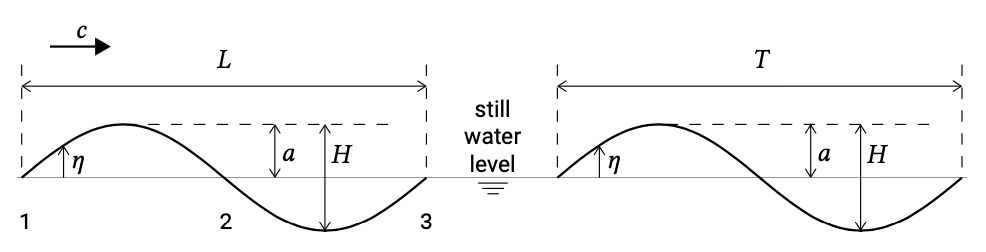
The simplest way of representing a wave is by a sine or cosine function: a regular variation of the water surface at a certain location. We will see later that such a sine wave is a solution to the linearised equations describing the water motion. In such a representation the temporal variation at one location is shown in the right hand side of Fig. 3.1.

The wave height \(H\) is the vertical distance between the crest and the trough of the wave and equals twice the amplitude \(a\) for a sinusoidal variation. The wave period \(T\) is the time the wave needs to pass the location, the inverse of which is the frequency \(f\), the number of waves passing a fixed location per unit time. When travelling in the ocean at a certain moment in time the wave can be seen as a similar sinusoidal variation of the water surface, see the left hand side of Fig. 3.1. The figure shows the wavelength \(L\) of the surface elevation deformation measured along the direction of wave propagation \(x\). The wavelength is the length a wave will travel in the wave period \(T\). The ratio between wave height and wavelength is called the wave steepness \(H/L\). The surface elevation \(\eta\) can be described by:

\[\eta = a \sin (\omega t - kx) = a \sin S(x, t)\]

where \(\omega\) is the angular frequency and \(k\) is the wavenumber according to:

\[k = \dfrac{2\pi}{L} \text{;}\ \ \ \ \omega = 2\pi f = \dfrac{2\pi}{T}\]

The deformations propagate with the wave speed \(c\):

\[c = \dfrac{L}{T} = \dfrac{\omega}{k}\]

In the linear (first order) approximation, wave propagation is merely a matter of movement of the wave form, not of mass. The water particles describe orbital or oscillatory motions at particle speed and remain at the same position on average. In Sect. 5.5.1 we will see that at second order there exists a non-zero net mass flux that becomes more important for larger wave amplitudes.

There are various ways to discern between the different types of ocean waves, viz. by:

• the disturbing force, i.e. their mechanism of generation;
• the restoring force, i.e. the mechanism that dampens the wave motion;
• the length of the wave (wavelength or equivalently wave period or frequency).

Figure 3.2: Sketch of the relative amounts of energy as a function of wave period in ocean waves. The top line gives the classification based on wavelength, the line below the classification based on the wave-generating force, and the bottom line the classification based on the restoring force. After Munk (1950) and Kinsman (1965).

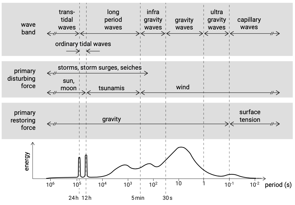
These different classifications are shown in Fig. 3.2 which shows the different ocean waves as a function of their wave period. In these lecture notes we will discuss the waves that are most important for our coastal system: wind waves (normal wind waves and longer storm waves), tides, tsunamis and storm surges. The energy level as indicated in Fig. 3.2 is a qualitative reflection of the amount of energy contained in these waves and their relative frequency of occurrence. Storm surges and tsunamis contain a lot of energy but are not as frequent as the ordinary wind waves. Therefore the energy contained in the wind wave range is higher.

Wind waves

Wind generated gravity waves have periods ranging from 1⁄4 s to 30 s. They are called gravity waves because gravity is the restoring force that dampens the wind wave motion by returning the particles to their average position in the water column. Local wind fields generate relatively short (order 10 s, larger for larger storms) random and irregular oscillations of the water surface that we call ‘sea’. These wind-generated oscillations can travel large distances away from their area of generation. They will then transform into longer, faster, lower and more regular ‘swell’ due to a process called frequency dispersion and frequency dependent damping (see Sect. 3.5.2). Capillary waves ( < 1/4 s ) can be seen as small ripples on the water surface, but they will die out really fast after the wind stops blowing. Their restoring force is surface tension. Infra-gravity waves are longer gravity waves with periods up to 5 minutes. Although deep water infra-gravity waves do exist, infra-gravity waves are mainly a shallow water phenomenon. In shallow water (groups of) wind waves can generate longer (30 s to 5 min) waves like surf beat, which has a period of say a few minutes (corresponding to the length of a wave group). This will be treated in Ch. 5. Note that the ratio of water depth to wavelength \(h/L\) or alternatively \(kh\) determines whether we are dealing with deep water (or short waves) and shallow water (or long waves).

Wind-generated gravity waves (sea and swell together) are the major supplier of energy to the coastal system. In this chapter therefore due attention is given to the generation and description of wind waves and their propagation in oceanic waters. The transformation they undergo when entering more shallow coastal waters will be treated in Ch. 5.

Tides

The tide is generated by the mutual gravitational attraction of the earth and the moon and of the earth and the sun. The frequencies of the tide are governed by the well- known movements of the earth, the moon and the sun and are mainly diurnal and semidiurnal (see the two spikes of the ordinary tidal waves in Fig. 3.2) and not continuous as with wind waves. The restoring force for long waves like tides is gravity, although the waves are influenced by Coriolis (see Intermezzo 3.1). The tide also attributes to shaping our coastal systems. Due to the once or twice daily rise and fall of the water level, the part of a coastal profile that is affected by waves changes during the tidal cycle; at high tide the waves will attack more shoreward portions of the profile than at low tide. In tidal basins intertidal areas between high and low water level act as storage areas for the water being brought in by the tide. The emptying and filling of the basin can give rise to large tidal currents in the inlets and keep the inlets open. Large tidal currents can also occur on open coasts around structures where convergence of the tidal current can be expected. The generation and propagation of the tide in oceanic waters will be treated in this Sects. 3.7 and 3.8. In Ch. 5 the specific processes in the coastal zone will be treated.

Intermezzo 3.1 Coriolis acceleration

Figure 3.3: As a result of the earth’s rotation any \(x, y, z\)-reference frame that is fixed to the earth’s surface also rotates.

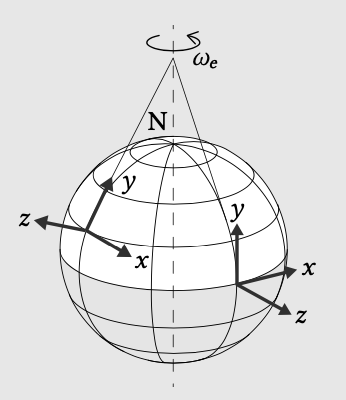
Since we are interested in water motion relative to the earth, our (numerical) models are mostly formulated in a frame of reference fixed to the earth’s surface. Generally, in such a reference frame, the \(z\)-axis is normal to the earth surface and outward directed, the \(x\)-axis points east and the \(y\)-axis points north (see Fig. 3.3). Because the earth rotates around its own axis (see Sect. 3.7.2), the chosen frame of reference also rotates (i.e. accelerates towards the centre of rotation).

Newton’s equations of motion are valid in an inertial frame of reference: a reference frame that does not accelerate, say a frame fixed to the distant stars. In order to make Newton’s equations of motion valid in our rotating, non-inertial frame of reference, we need to introduce ‘fictitious’ centrifugal^a and Coriolis forces. These forces are called ‘pseudo-’ or ‘fictitious’ forces since they do not arise from any physical interaction but from the choice of a non-inertial reference frame.

The Coriolis force is named after Coriolis who first described it in the first half of the 19^th century. As will be explained below, this force acts on every moving particle in the rotating reference frame, at right angles to the direction of motion, to the right in the Northern Hemisphere (NH) and to the left in the Southern Hemisphere (SH). Hence, the Coriolis effect causes air and water currents in the Northern Hemisphere to deflect to the right, and in the Southern Hemisphere to the left.

Figure 3.4: Gnomonic map projection of latitudinal lines. In such a projection great circles (the shortest distance between two locations on a spherical object) are displayed as straight lines and directions are preserved. The \(x,y\)-plane turns anti-clockwise in the NH and clockwise in the SH.

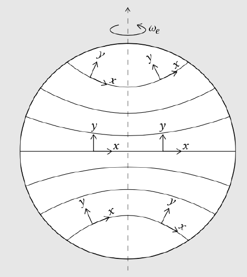
In the Northern Hemisphere the rotation of the reference frame implies an anti-clockwise rotation of the \(x,y\)-plane, the horizontal plane tangent to the earth’s surface (see Fig. 3.4). When observing motion in a horizontal plane that is turning anti-clockwise, a particle travelling in a straight line (as seen from the stars) appears to be turning clockwise. To describe this deflection to the right, a Coriolis force acting to the right must be introduced in Newton’s equations of motion.

In the Southern Hemisphere the \(x,y\)-plane has rotated clockwise after some time, such that the Coriolis force acts to the left (or anti-clockwise). At the equator the Coriolis force is zero^b. This is because at the equator the earth’s surface lies in a plane parallel to the earth’s axis of rotation. Hence, the earth’s rotation vector \(\omega_e\) (see Fig. 3.4) has no component perpendicular to the earth surface and the angular velocity of the horizontal plane (the rate at which the \(x,y\) axes change direction) is zero. Going from the equator to the poles, the rotation vector is less and less parallel to the earth’s surface until at the poles it is entirely perpendicular to the earth’s surface. Hence, the horizontal (i.e. parallel to the earth surface) Coriolis forces are zero at the equator and largest at the poles.

At a latitude \(\varphi\), the earth-normal component of the rotation vector is \(\omega_e \sin \varphi\). It represents the angular velocity of the horizontal plane (the rate at which the \(x,y\)-coordinate axes change direction). The Coriolis force is proportional to 1) the angular velocity of the horizontal plane; and to 2) the velocity of the moving particle or object in the rotating reference frame. It can be shown that the Coriolis acceleration (or Coriolis force per unit mass) to the right of the velocity \(V\) reads:

\[a_c = fV = 2\omega_e \sin \varphi V\]

where

\(a_c\)	Coriolis acceleration	\(m/s^2\)
\(f\)	Coriolis parameter	\(1/s\)
\(\omega_e\)	angular velocity of the earth	\(rad/s\)
\(V\)	current velocity	\(m/s\)
\(\varphi\)	latitude (positive in NH and negative in SH)	°

The earth angular velocity \(\omega_e = 72.9 \times 10^{-6}\ rad/s\) is based on sidereal day, i.e. the time needed by the earth to complete a rotation around its axis, 23 hours and 56 minutes. With the latitude and hence the Coriolis parameter positive in the Northern Hemisphere and negative in the Southern Hemisphere, the direction of the acceleration is to starboard in the Northern Hemisphere and to port in the Southern Hemisphere. Its magnitude is largest at the poles where \(|\sin \varphi | = 1\) and zero at the equator where \(\sin \varphi = 0\). At mid-latitudes (say \(\varphi \approx\) 45°) we have \(f \approx 10^{-4} s^{-1}\). However, in practice, in numerical models covering not too large areas the parameter �� can be assumed to be a constant.

Whether the Coriolis deflection is significant relative to inertia can be determined by the Rossby number, which is given by:

\[R = \dfrac{V}{|f|L}\]

with \(L\) is the length scale of the motion. The Rossby number can be seen as the ratio between the inertial forces and Coriolis forces, see also Sect. 3.8.3. For Rossby numbers of order 1 and smaller Coriolis deflection is important, which is for instance the case for large-scale motions such as tides. To describe tidal motion, the Coriolis acceleration must be introduced in Newton’s equations of motion. How this is done is discussed in Sect. 3.8.3.

---

a. The ‘fictitious’ centrifugal force (directed away from the axis of rotation) does not seem to be invoked by any true force since for an observer in the rotating reference frame the centripetal acceleration of the earth (towards the rotation axis) is hidden.

b. Or more precisely: the horizontal components of the Coriolis force (in the \(x,y\)-plane) are zero. Coriolis force acts in a direction perpendicular to the rotation axis of the earth, which is normal to the earth’s surface at the equator.

Tsunamis

Also indicated in Fig. 3.2, tsunamis are a specific type of wave not caused by wind but by large, impulsive displacement of the sea level. The disturbance of the water surface is usually triggered by underwater earthquakes or underwater volcanic eruptions. The surface disturbance travels away from its origin in a pattern comparable with the patterns generated by the landing of a pebble in a pond. In deep water, tsunamis are not visible because they are small in height and very long in wavelength (periods ranging from 5 min to 60 min). They may grow to devastating proportions at the coast where the water is shallow. This effect of tsunamis will be discussed in Ch. 5, whereas the propagation of tsunamis through the oceans is treated in Sect. 3.5.2. Approximately every 15 years a destructive, ocean-wide tsunami occurs.

Tsunami warning systems are in place, which recognise either seismic activity that can potentially lead to a tsunami or unusual water level variations.

Storm surges

Storm surges are elevations of the water surface with time and spatial scales equal to those of the large storm fields that generate them. They are generated by the low atmospheric pressure and high wind speeds in a storm field. The wavelength and period are generally slightly shorter than those of tides. Storm surges can cause severe flooding because the water will pile up against the coast when they approach the coast (see Ch. 5). Examples are the flooding of New Orleans due to the storm surge associated with hurricane Katrina in 2005, the regular cyclone-induced floodings of Bangladesh and the 1953 storm surge in the Netherlands (see Sect. 1.4.6).