
1.4.2: Cross-shore profile
- Page ID
- 16259

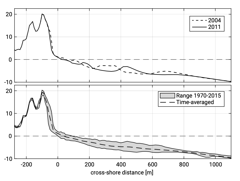
The upper panel of Fig. 1.2 shows the shape of a cross-section (called cross-shore pro- file) as measured perpendicular to a sandy coast at two moments in time. The lower panel shows the variation in time around an average profile. Please notice that the vertical and horizontal scales of the plot are quite different. Dunes, beach and a part of the so-called shoreface can be discerned. The actual slope of the dune face is 1:3 to 1:4. The slope of the beach is decreasing from the upper part of the beach near the foot of the dunes (1:20) towards the sea; near the waterline the slope is approximately 1:50. At the shoreface some (breaker) bars are present. The average bottom slope becomes flatter with longer distance from the waterline. At the seaward end of the plot (water depth: MSL −10 m) the slope is approximately 1:125.
The water level as indicated in Fig. 1.2 reflects the Mean Sea Level (MSL). This is the sea level averaged over a period of time such as a month or a year such that periodic sea-level changes e.g. due to waves and tides are averaged out. In the Netherlands, MSL is approximately equal to the Dutch reference level called NAP (Normaal Amsterdams Peil in Dutch)1. The seabed consists of sandy material that generally fines when going further offshore. A typical grain size for a sandy coast is \(D_{50} = 200 \ \mu m\); 150 million of these particles fit into a volume of 1 litre!
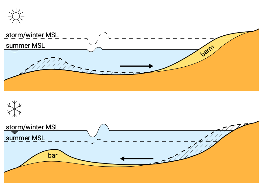
Under the influence of waves the position of the coastline (say represented by the intersection of MSL and the profile) will continuously change. Variations will take place on the timescale of storms and seasons. During storms, high and long waves cause erosion of the beach. This sediment is deposited in the surf zone (the zone where the waves are breaking). A typical storm profile therefore has a narrow beach and a relatively flat slope. Seasonality is especially evident in the Northern Hemisphere which experiences a large number of storms in winter (see Sect. 4.3.1). Hence, a storm profile is also often called a winter profile. During storms high water levels can also cause dune erosion and flooding (see Sect. 1.4.6). In summer the sand is moved back towards the beach and dunes by lower and shorter waves. This cross-shore transport of sediment causes oscillations of the coastline (Fig. 1.3), but in principle the mean position of the coastline does not change. The mean position of the coastline will only change in the case of a structural loss or gain of sediment; structural erosion may occur when sand disappears in offshore canyons or in the alongshore direction (Sect. 1.4.3). Seasonal variations are relevant to tourism (beach width) or the safety of property close to the brink (highest point) of the dune.
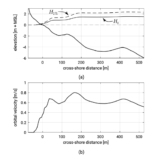
Suppose that irregular waves (also called random waves) approach the coast perpendicularly with a significant deep water wave height of \(H_{s, 0} = 2\ m\) and a peak period of \(T_p = 10\ s\) (for the definitions see Sects. 3.4.2 and 3.4.3). The wave height distribution along the profile (Fig. 1.4a) can be calculated with numerical models based on a spectral energy or action balance (Sects. 3.5.3 and 5.2.1). Notice that the wave height in Fig. 1.4a reduces gradually when the waves approach the waterline. This is due to energy dissipation due to (partial) wave breaking and bottom friction.
In Fig. 1.4b the maximum horizontal components of the orbital velocities near the bed are plotted as a function of the position in the cross-shore profile. Notice the rather large magnitudes (\(>1\ m/s\) at many positions). Realizing that the critical velocity to initiate motion in uniform flow for particles with \(D_{50} = 200 \ \mu m\) is approximately \(0.2\ m/s\) (see Sect. 6.3), one may understand that the waves of Fig. 1.4a are able to stir up many particles in the cross-shore profile. The turbulence generated by breaking waves is very effective in keeping those particles away from the bed. The particles can subsequently be transported by for instance wave-generated and tidal currents (see Ch. 5). Also asymmetric waves can give a net sediment transport. Chapter 6 discusses sediment transport in general, whereas Ch. 7 focuses on cross-shore transport. Both the magnitude and direction (onshore-offshore) of the cross-shore transport may change depending on the local hydrodynamic conditions.
Often the effect of cross-shore oscillations is assumed to average out on the longer term. In those cases structural trends in coastline position are due to sediment transport along the coast (or more correctly due to gradients in longshore transport, as we will see in Sect. 1.4.3). Nevertheless, some important practical problems are related to changes in the shape of the profile with time (e.g. dune erosion and the behaviour of beach and shoreface nourishments)
1. Recently, MSL has been around NAP + 0.06 m in the Netherlands.