17.5: Gap Winds

17.5.1. Basics

During winter in mountainous regions, sometimes the synoptic-scale weather pattern can move very cold air toward a mountain range. The cold air is denser than the warm overlying air, so buoyancy opposes rising motions in the cold air. Thus, the mountain range is a barrier that dams cold air behind it.

Figure 17.19 Geography of southwestern British Columbia, Canada, and northwestern Washington, USA, illustrating mountain gaps. Higher elevations are shown as darker greys, with the highest peaks 3,000 to 4,000 m above sea level. Ocean and very-lowelevation-land areas are white. Lower-elevation fjords, straits, and river valleys (i.e., gaps) appear as filaments of white or light-grey across the dark-shaded mountain range. In winter, sometimes very cold arctic air can pool in the Interior Plateau northeast of the Coast Mountains.

Figure 17.20 Cold air flow through a short gap.

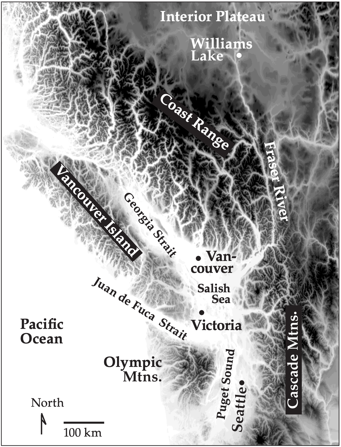
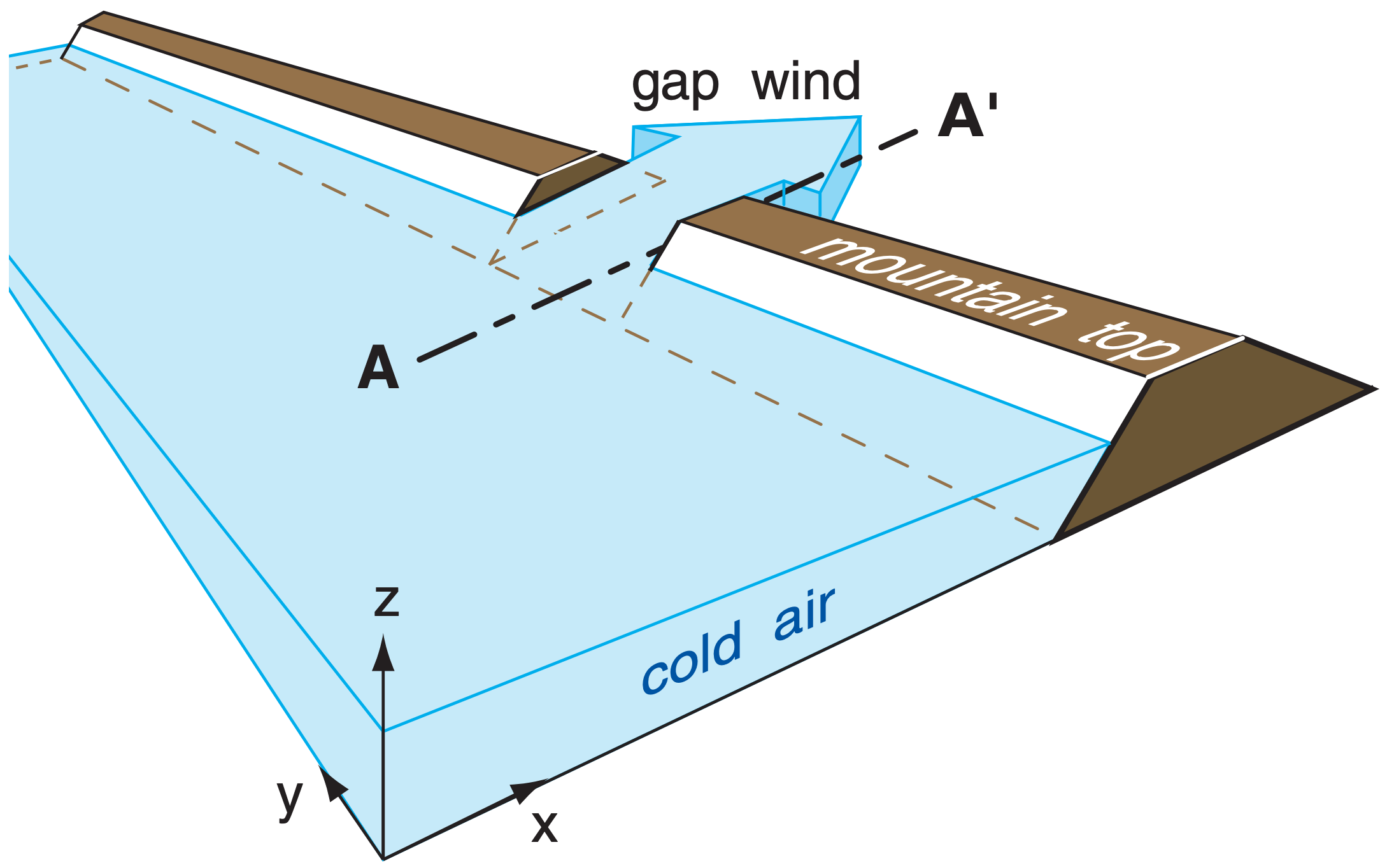
However, river valleys, fjords, straits, and passes (Fig. 17.19) are mountain gaps through which the cold air can move as gap winds (Fig. 17.20). Gap wind speeds of 5 to 25 m s^–1 have been observed, with gusts to 40 m s^–1. Temperature jumps at the top of the cold-air layer in the 5 to 10°C range are typical, while extremes of 15°C have been observed. Gap flow depths of 500 m to over 2 km have been observed. In any locale, the citizens often name the gap wind after their town or valley.

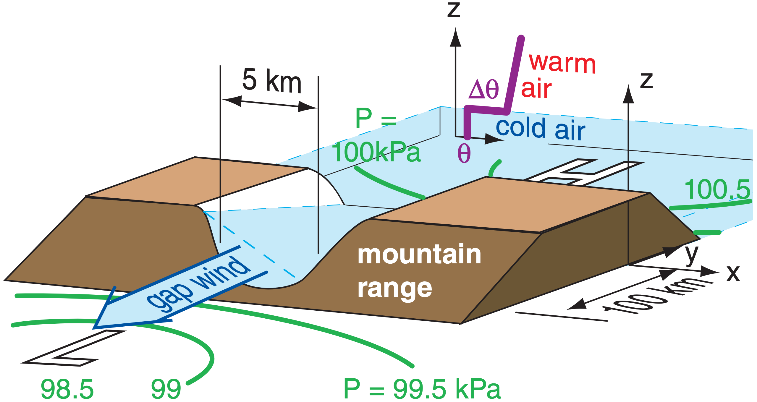
The cold airmass dammed on one side of the mountain range often has high surface pressure (H), as explained in the Hydrostatic Thermal Circulation section of the General Circulation chapter. When synoptic low-pressure centers (L) approach the opposite side of the mountain range, a pressure gradient of order (0.2 kPa)/(100 km) forms across the range that can drive the gap wind. Gap winds can also be driven by gravity, as cold air is pulled downslope through a mountain pass.

Divide gap flow into two categories based on the gap geometry: (1) short gaps, and (2) long gaps. Long gaps are ones with a gap width (order of 2 - 20 km) that is much less than the gap length (order of 100 km). Coriolis force is important for flow through long gaps, but is small enough to be negligible in short gaps.

17.5.2. Short-gap Winds

Figure 17.21 Cold air flow through a short gap. Vertical slice inside the gap, along section A - A’ from the previous figure. A series of 3 hydraulic jumps are shown in this idealization.

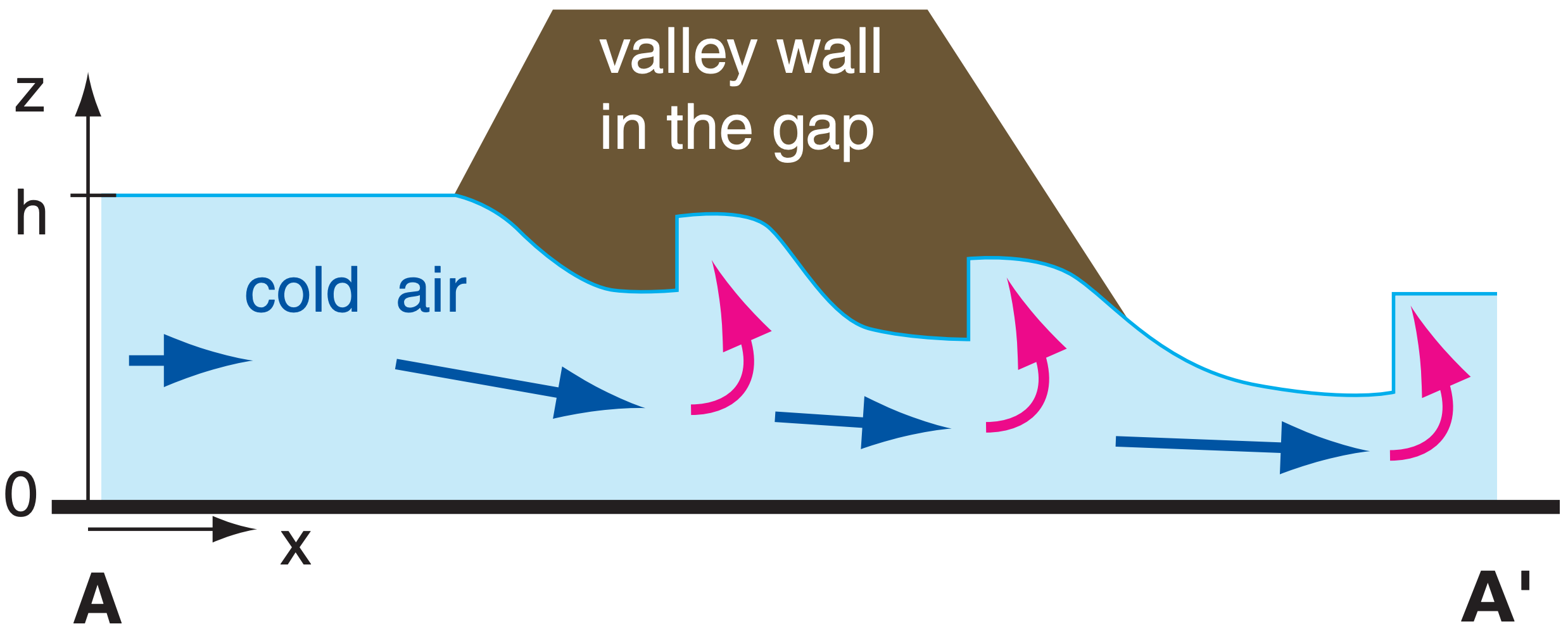
For short gaps, you can neglect Coriolis force and use open-channel hydraulics. Although the gap-wind speed could range from subcritical to supercritical, observations suggest that one or more hydraulic jumps (Fig. 17.21) are usually triggered in the supercritical regions due to irregularities in the valley shape, or by obstacles, similar to hydraulic jumps you can see in irregular river channels. The resulting turbulence in the hydraulic jumps causes extra drag, slowing the wind to its critical value.

The net result is that many gap winds are likely to have maximum speeds nearly equal to their critical value: the speed that gives F_r = 1. Using this in the definition of the Froude number allows us to solve for the likely maximum gap wind speed through gaps short enough that Coriolis force is not a factor:

\(\ \begin{align} M_{g a p \max }=\left[|g| \cdot \dfrac{\Delta \theta_{v}}{T_{v}} \cdot h\right]^{1 / 2}\tag{17.25}\end{align}\)

17.5.3. Long-gap Winds

Sample Application

Cold winter air of virtual potential temperature –5°C and depth 200 m flows through an irregular short mountain pass. The air above has virtual potential temperature 10°C. Find the max likely wind speed through the short gap.

Find the Answer

Given: ∆θ_v = 15°C = 15K, h = 200 m.

Find: M_{gap max} = ? m s^–1

For a 2-layer air system, use eq. (17.25):

M_{gap max} = [(9.8 m·s^–2)·(15K)·(200m)/(267K)]^1/2 = 10.5 ms^–1

Check: Units OK. Magnitude OK.

Exposition: Because of the very strong temperature jump across the top of the cold layer of air and the correspondingly faster wave group speed, faster gap flow speeds are possible. Speeds any faster than this would cause an hydraulic jump, which would increase turbulent drag and slow the wind back to this wind speed.

17.5.3. Long-gap Winds

For long gaps, examine the horizontal forces (including Coriolis force) that act on the air. Consider a situation where the synoptic-scale isobars are nearly parallel to the axis of the mountain range (Fig. 17.22), causing a pressure gradient across the mountains.

Figure 17.22 Scenario for gap winds in the N. Hemisphere in long valleys, with cold air (light blue) dammed behind a mountain range (brown). High pressure (H) is in the cold air, and low pressure (L) is at the opposite side of the mountains. Thick curved green lines are sea-level isobars around the synoptic-scale pressure centers. The vertical profile of potential temperature θ is plotted (purple).

For long narrow valleys this synoptic-scale crossmountain pressure gradient is unable to push the cold air through the gap directly from high to low pressure, because Coriolis force tends to turn the wind to the right of the pressure gradient. Instead, the cold air inside the gap shifts its position to enable the gap wind, as described next.

Figure 17.23 An enlargement of just the mountain gap portion of the previous figure. (a)-(c) Oblique view showing evolution of the cold air (light blue) in the gap. (a’)-(c’) Plan view (looking down from above) showing the corresponding forces acting on a cold air parcel as a gap wind forms (see text for details).

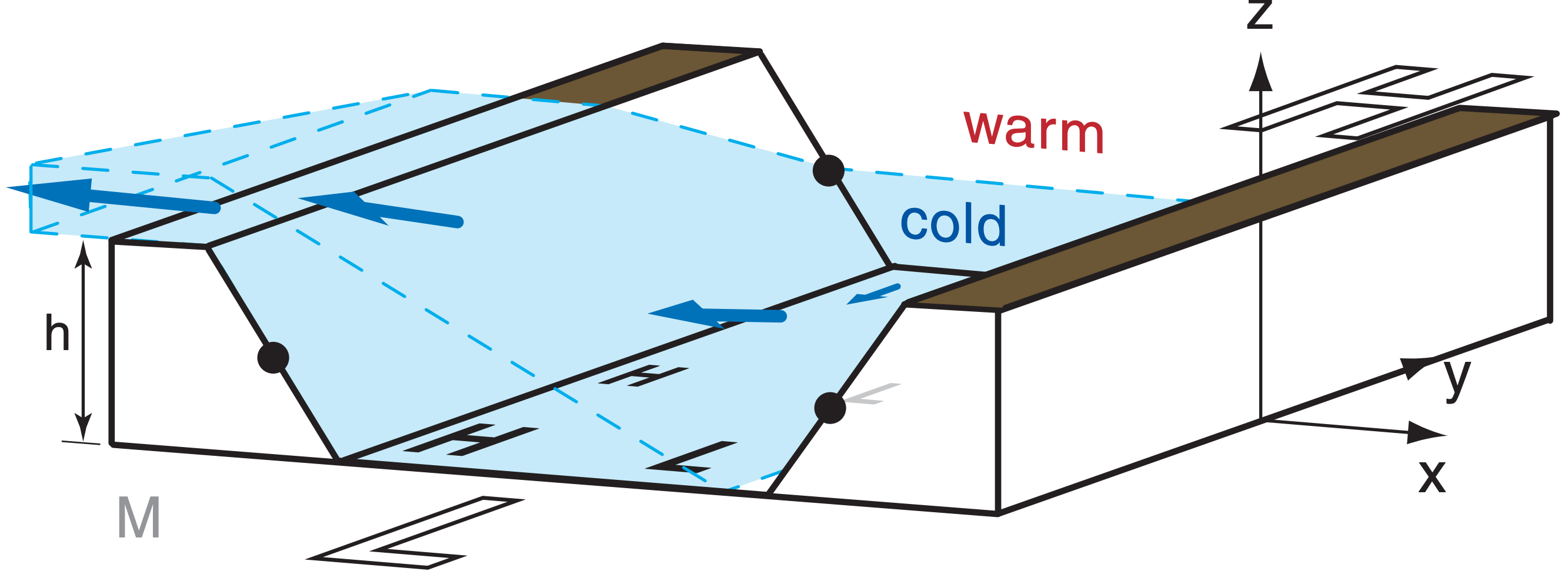
Fig. 17.23 idealizes how this wind forms in the N. Hemisphere. Cold air (light grey in Fig. 17.23a) initially at rest in the gap feels the synoptically imposed pressure-gradient force F_PGs along the valley axis, and starts moving at speed M (shown with the short dark-blue arrow in Fig. 17.23a’) toward the imposed synoptic-scale low pressure (L) on the opposite side of the gap. At this slow speed, both Coriolis force (F_CF) and turbulent drag force (F_TD) are correspondingly small (Fig. 17.23a’). The sum (black-andwhite dotted arrow) of all the force vectors (black) causes the wind to turn slightly toward its right in the N. Hemisphere and to accelerate into the gap.

This turning causes the cold air to “ride up” on the right side of the valley (relative to the flow direction, see Fig. 17.23b). It piles up higher and higher as the gap wind speed M increases. But cold air is denser than warm. Thus slightly higher pressure (small dark-grey H) is under the deeper cold air, and slightly lower pressure (small dark-grey L) is under the shallower cold air. The result is a cross-valley mesoscale pressure-gradient force F_PGm per unit mass m (Fig. 17.23b’) at the valley floor of:

\(\ \begin{align} \dfrac{F_{P G m}}{m}=-\dfrac{1}{\rho} \cdot \dfrac{\Delta P_{m}}{\Delta x}=-|g| \cdot \dfrac{\Delta \theta_{v}}{T_{v}} \cdot \dfrac{\Delta z}{\Delta x}\tag{17.26}\end{align}\)

where ∆z/∆x is the cross-valley slope of the top of the cold-air layer, ∆P_m/∆x is the mesoscale pressure gradient across the valley, ∆θ_v is the virtual potential temperature difference between the cold and warm air, T_v is an average virtual temperature (Kelvin), |g| = 9.8 m·s^–2 is the magnitude of gravitational acceleration, and ρ is the average air density.

When this new pressure gradient force is vectoradded to the larger drag and Coriolis forces associated with the moderate wind speed M, the resulting vector sum of forces (dotted white-and-black vector; Fig. 17.23b’) begins to turn the wind to become almost parallel to the valley axis.

Gap-wind speed M increases further down the valley (Fig. 17.23c and c’), with the gap-wind cold air hugging the right side of the valley. In the alongvalley direction (the –y direction in Figs. 17.23), the synoptic pressure gradient force F_PGs is often larger than the opposing turbulent drag force FTD, allowing the air to continue to accelerate along the valley, reaching its maximum speed near the valley exit. The antitriptic wind results from a balance of drag and synoptic-scale pressure-gradient forces. Similar gap winds are sometimes observed in the Juan de Fuca Strait (Fig. 17.19), with the fastest gap winds near the west exit region of the strait.

In the cross-valley direction, Coriolis force F_CF nearly balances the mesoscale pressure gradient force F_PGm. These last two forces define a mesoscale “gap-geostrophic wind” speed G_m parallel to the valley axis:

\(\ \begin{align}G_{m}=\left|\dfrac{g}{f_{c}} \cdot \dfrac{\Delta \theta_{v}}{T_{v}} \cdot \dfrac{\Delta z}{\Delta x}\right|\tag{17.27}\end{align}\)

The actual gap wind speeds are of the same order of magnitude as this gap-geostrophic wind.

The synoptic-scale geostrophic wind on either side of the mountain range is nearly equal to the synoptic-scale geostrophic wind well above the mountain (G, in Fig. 17.23a). These synoptic winds are at right angles to the mesoscale gap-geostrophic wind.

Figure 17.24 Gap winds can overtop the valley side walls if these walls are too low, or if the temperature difference between cold and warm layers of air is too small.

The maximum possible gap wind speed is given by the equation above, but with ∆z replaced with the height h of the valley walls above the valley floor. If either h or ∆θ_v are too small, then some of the cool air can ride far enough up the valley wall to escape over top of the valley walls (Fig. 17.24), and the resulting gap winds are weaker. Gap winds occur more often in winter, when cold valley air causes large ∆θ_v.

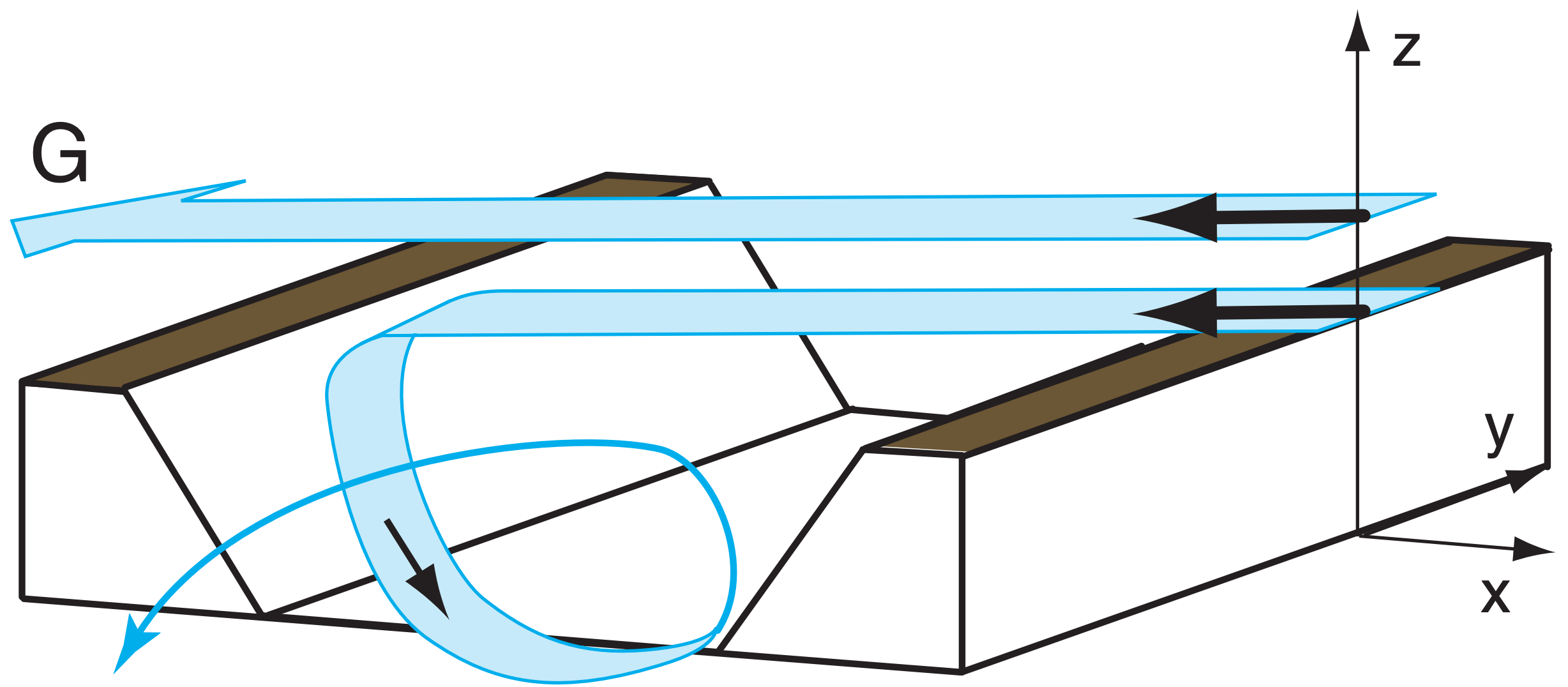
For a case where ∆θ_v is near zero (i.e., near-neutral static stability), the synoptic-scale geostrophic wind dominates. The vector component of G along the valley axis can appear within the valley as a channeled wind parallel to the valley axis. However, the cross-valley component of G can create strong turbulence in the valley (due to cavity, wake, and mountain-wave effects described later in this chapter). These components combine to create a turbulent corkscrew motion within the valley (Fig. 17.25).

Figure 17.25 Without a layer of cold air near the surface, the cross-valley component of synoptic-scale geostrophic wind can create turbulent corkscrew motions and channeling of wind in the valley.

Sample Application

What long-gap wind speed can be supported in a strait 10 km wide through mountains 0.5 km high? The cold air is 4°C colder than the overlying 292 K air.

Find the Answer

Given: h = ∆z = 0.5 km, ∆x = 10 km, ∆θ_v = 4°C = 4 K, T_v = 0.5·(288K + 292K) = 290K.

Find: G_m = ? m s^–1

Assume: f_c = 10^–4 s^–1.

Use eq. (17.27):

G_m = |(9.8 m·s^–2/ 10^–4 s^–1)·(4K/290K)·(0.5km/10km)| = 67 ms^–1.

Check: Units OK. Magnitude seems too large.

Exposition: The unrealistically large magnitude might be reached if the strait is infinitely long. But in a finite-length strait, the accelerating air would exit the strait before reaching this theoretical wind speed.

We implicitly assumed that the air was relatively dry, allowing T_v ≈ T, and ∆θ_v ≈ ∆θ. If humidity is larger, then you should be more accurate when calculating virtual temperatures. Also, as the air accelerates within the valley, mass conservation requires that the air depth ∆z decreases, thereby limiting the speed according to eq. (17.27).