Geosciences LibreTexts

11.10: Horizontal Circulation

  • Page ID
    10210
  • \( \newcommand{\vecs}[1]{\overset { \scriptstyle \rightharpoonup} {\mathbf{#1}} } \)

    \( \newcommand{\vecd}[1]{\overset{-\!-\!\rightharpoonup}{\vphantom{a}\smash {#1}}} \)

    \( \newcommand{\id}{\mathrm{id}}\) \( \newcommand{\Span}{\mathrm{span}}\)

    ( \newcommand{\kernel}{\mathrm{null}\,}\) \( \newcommand{\range}{\mathrm{range}\,}\)

    \( \newcommand{\RealPart}{\mathrm{Re}}\) \( \newcommand{\ImaginaryPart}{\mathrm{Im}}\)

    \( \newcommand{\Argument}{\mathrm{Arg}}\) \( \newcommand{\norm}[1]{\| #1 \|}\)

    \( \newcommand{\inner}[2]{\langle #1, #2 \rangle}\)

    \( \newcommand{\Span}{\mathrm{span}}\)

    \( \newcommand{\id}{\mathrm{id}}\)

    \( \newcommand{\Span}{\mathrm{span}}\)

    \( \newcommand{\kernel}{\mathrm{null}\,}\)

    \( \newcommand{\range}{\mathrm{range}\,}\)

    \( \newcommand{\RealPart}{\mathrm{Re}}\)

    \( \newcommand{\ImaginaryPart}{\mathrm{Im}}\)

    \( \newcommand{\Argument}{\mathrm{Arg}}\)

    \( \newcommand{\norm}[1]{\| #1 \|}\)

    \( \newcommand{\inner}[2]{\langle #1, #2 \rangle}\)

    \( \newcommand{\Span}{\mathrm{span}}\) \( \newcommand{\AA}{\unicode[.8,0]{x212B}}\)

    \( \newcommand{\vectorA}[1]{\vec{#1}}      % arrow\)

    \( \newcommand{\vectorAt}[1]{\vec{\text{#1}}}      % arrow\)

    \( \newcommand{\vectorB}[1]{\overset { \scriptstyle \rightharpoonup} {\mathbf{#1}} } \)

    \( \newcommand{\vectorC}[1]{\textbf{#1}} \)

    \( \newcommand{\vectorD}[1]{\overrightarrow{#1}} \)

    \( \newcommand{\vectorDt}[1]{\overrightarrow{\text{#1}}} \)

    \( \newcommand{\vectE}[1]{\overset{-\!-\!\rightharpoonup}{\vphantom{a}\smash{\mathbf {#1}}}} \)

    \( \newcommand{\vecs}[1]{\overset { \scriptstyle \rightharpoonup} {\mathbf{#1}} } \)

    \( \newcommand{\vecd}[1]{\overset{-\!-\!\rightharpoonup}{\vphantom{a}\smash {#1}}} \)

    \(\newcommand{\avec}{\mathbf a}\) \(\newcommand{\bvec}{\mathbf b}\) \(\newcommand{\cvec}{\mathbf c}\) \(\newcommand{\dvec}{\mathbf d}\) \(\newcommand{\dtil}{\widetilde{\mathbf d}}\) \(\newcommand{\evec}{\mathbf e}\) \(\newcommand{\fvec}{\mathbf f}\) \(\newcommand{\nvec}{\mathbf n}\) \(\newcommand{\pvec}{\mathbf p}\) \(\newcommand{\qvec}{\mathbf q}\) \(\newcommand{\svec}{\mathbf s}\) \(\newcommand{\tvec}{\mathbf t}\) \(\newcommand{\uvec}{\mathbf u}\) \(\newcommand{\vvec}{\mathbf v}\) \(\newcommand{\wvec}{\mathbf w}\) \(\newcommand{\xvec}{\mathbf x}\) \(\newcommand{\yvec}{\mathbf y}\) \(\newcommand{\zvec}{\mathbf z}\) \(\newcommand{\rvec}{\mathbf r}\) \(\newcommand{\mvec}{\mathbf m}\) \(\newcommand{\zerovec}{\mathbf 0}\) \(\newcommand{\onevec}{\mathbf 1}\) \(\newcommand{\real}{\mathbb R}\) \(\newcommand{\twovec}[2]{\left[\begin{array}{r}#1 \\ #2 \end{array}\right]}\) \(\newcommand{\ctwovec}[2]{\left[\begin{array}{c}#1 \\ #2 \end{array}\right]}\) \(\newcommand{\threevec}[3]{\left[\begin{array}{r}#1 \\ #2 \\ #3 \end{array}\right]}\) \(\newcommand{\cthreevec}[3]{\left[\begin{array}{c}#1 \\ #2 \\ #3 \end{array}\right]}\) \(\newcommand{\fourvec}[4]{\left[\begin{array}{r}#1 \\ #2 \\ #3 \\ #4 \end{array}\right]}\) \(\newcommand{\cfourvec}[4]{\left[\begin{array}{c}#1 \\ #2 \\ #3 \\ #4 \end{array}\right]}\) \(\newcommand{\fivevec}[5]{\left[\begin{array}{r}#1 \\ #2 \\ #3 \\ #4 \\ #5 \\ \end{array}\right]}\) \(\newcommand{\cfivevec}[5]{\left[\begin{array}{c}#1 \\ #2 \\ #3 \\ #4 \\ #5 \\ \end{array}\right]}\) \(\newcommand{\mattwo}[4]{\left[\begin{array}{rr}#1 \amp #2 \\ #3 \amp #4 \\ \end{array}\right]}\) \(\newcommand{\laspan}[1]{\text{Span}\{#1\}}\) \(\newcommand{\bcal}{\cal B}\) \(\newcommand{\ccal}{\cal C}\) \(\newcommand{\scal}{\cal S}\) \(\newcommand{\wcal}{\cal W}\) \(\newcommand{\ecal}{\cal E}\) \(\newcommand{\coords}[2]{\left\{#1\right\}_{#2}}\) \(\newcommand{\gray}[1]{\color{gray}{#1}}\) \(\newcommand{\lgray}[1]{\color{lightgray}{#1}}\) \(\newcommand{\rank}{\operatorname{rank}}\) \(\newcommand{\row}{\text{Row}}\) \(\newcommand{\col}{\text{Col}}\) \(\renewcommand{\row}{\text{Row}}\) \(\newcommand{\nul}{\text{Nul}}\) \(\newcommand{\var}{\text{Var}}\) \(\newcommand{\corr}{\text{corr}}\) \(\newcommand{\len}[1]{\left|#1\right|}\) \(\newcommand{\bbar}{\overline{\bvec}}\) \(\newcommand{\bhat}{\widehat{\bvec}}\) \(\newcommand{\bperp}{\bvec^\perp}\) \(\newcommand{\xhat}{\widehat{\xvec}}\) \(\newcommand{\vhat}{\widehat{\vvec}}\) \(\newcommand{\uhat}{\widehat{\uvec}}\) \(\newcommand{\what}{\widehat{\wvec}}\) \(\newcommand{\Sighat}{\widehat{\Sigma}}\) \(\newcommand{\lt}{<}\) \(\newcommand{\gt}{>}\) \(\newcommand{\amp}{&}\) \(\definecolor{fillinmathshade}{gray}{0.9}\)

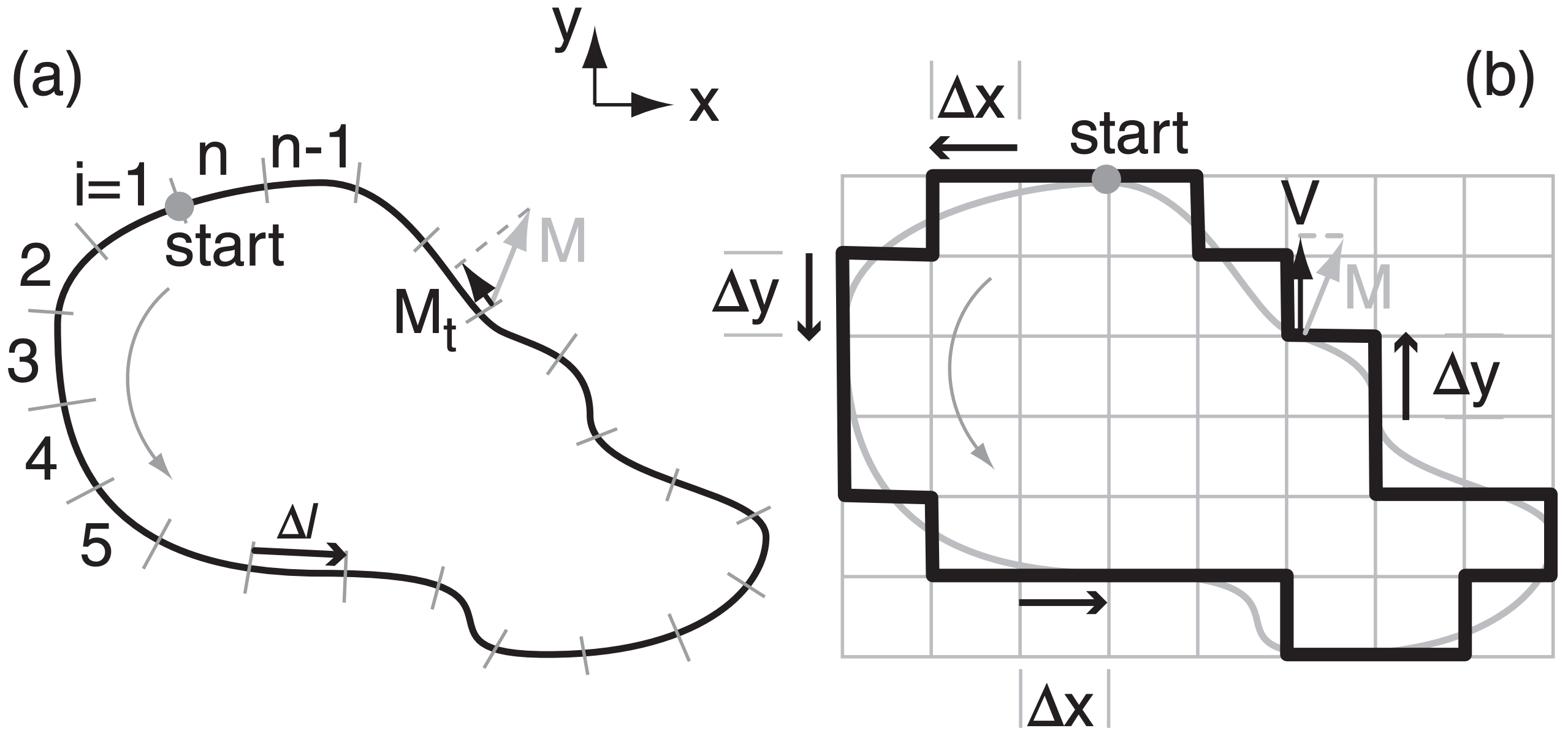
    Consider a closed shape of finite area (Fig. 11.47a). Pick any starting point on the perimeter, and hypothetically travel counterclockwise around the perimeter until you return to the starting point. As you travel each increment of distance ∆l, observe the local winds along that increment, and get the average tangential component of wind velocity Mt.
    Screen Shot 2020-03-04 at 12.15.08 AM.png
    Figure 11.47 Method for finding the circulation. M is the wind vector. Mt and V are projections onto the perimeter. (a) Stepping in increments of ∆l around an arbitrary shape. (b) Stepping around a Cartesian (gridded) approximation to the shape in (a).

    The horizontal circulation C is defined as the product of this tangential velocity times distance increment, summed over all the increments around the whole perimeter:

    \(\ \begin{align} C=\sum_{i=1}^{n}\left(M_{t} \cdot \Delta l\right)_{i}\tag{11.28}\end{align}\)

    where i is the index of each increment, and n is the number of increments needed to complete one circuit around the perimeter. Take care that the sign of Mt is such that it is positive if the tangential wind is in the same direction as you are traveling, and negative if opposite. The units of circulation are m2·s–1.

    If we approximate the perimeter by Cartesian line segments (Fig. 11.47b), then eq. (11.28) becomes:

    \(\ \begin{align} C=\sum_{i=1}^{n}(U \cdot \Delta x+V \cdot \Delta y)_{i}
    \tag{11.29}\end{align}\)

    The sign of ∆x is (+) if you travel in the positive x-direction (toward the East), and (–) if opposite. Similar rules apply for ∆y (+ toward North).

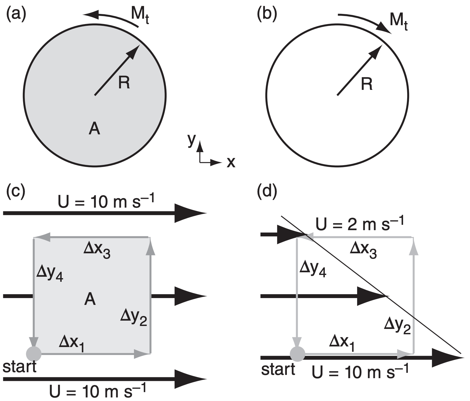
    To better understand circulation, consider idealized cases (Figs. 11.48a & b). For winds of tangential velocity Mt rotating counterclockwise around a circle of radius R, the circulation is C = 2πR·Mt. For clockwise circular rotation, the circulation is C = –2πR·Mt , namely, the circulation value is negative. From these two equations, we see that a fast speed around a small circle (such as a tornado) can give the same circulation magnitude as a slower speed around a larger circle (e.g., a mid-latitude cyclone).
    Screen Shot 2020-03-04 at 12.19.07 AM.png
    Figure 11.48 Circulation examples. (a) Counterclockwise rotation around a circle. (b) Clockwise rotation around a circle. (c) Uniform wind. (d) Uniform shear. Area A enclosed by circulation is shaded.

    Consider two more cases (Figs. 11.48c & d). For a circuit in a constant wind field of any speed, the circulation is C = 0. For a circuit within a region of uniform shear such as ∆U/∆y, the circulation is C = –(∆U/∆y)·(∆y·∆x). Comparing these last two cases, we see that the wind speed is irrelevant for the circulation, but the wind shear is very important.

    In the last equation above, (∆y·∆x) = A is the area enclosed by the circulation of Fig. 11.48d. In general, for uniform U and V shear across a region, the horizontal circulation is:

    \(\ \begin{align} C=\left(\frac{\Delta V}{\Delta x}-\frac{\Delta U}{\Delta y}\right) \cdot A\tag{11.30}\end{align}\)

    But the term in parentheses is the relative vorticity ζr . This gives an important relationship between horizontal circulation and vorticity:

    \(\ \begin{align} C=\zeta_{r} \cdot A\tag{11.31}\end{align}\)

    Vorticity is defined at any one point in a fluid, while circulation is defined around a finite-size area. Thus, eq. (11.31) is valid only in the limit as A becomes small, or for the special case of a fluid having uniform vorticity within the whole circulation area.

    The horizontal circulation C defined by eq. (11.30 & 11.31) is also known as the relative circulation Cr . An absolute circulation Ca can be defined as

    \(\ \begin{align} C_{a}=\left(\zeta_{r}+f_{c}\right) \cdot A\tag{11.32}\end{align}\)

    where fc is the Coriolis parameter. The absolute circulation is the circulation that would be seen from a fixed point in space looking down on the atmosphere rotating with the Earth.

    For the special case of a frictionless barotropic atmosphere (where isopycnics are parallel to isobars), Kelvin’s circulation theorem states that Ca is constant with time.

    For a more realistic baroclinic atmosphere containing horizontal temperature gradients, the Bjerknes circulation theorem:

    \(\ \begin{align} \frac{\Delta C_{r}}{\Delta t}=-\sum_{i=1}^{n}\left(\frac{\Delta P}{\rho}\right)_{i}-f_{c} \cdot \frac{\Delta A}{\Delta t}\tag{11.33}\end{align}\)

    says relative circulation varies with the torque applied to the fluid (via the component of pressure forces in the direction of travel, summed around the perimeter of the circulation area) minus the Earth’s rotation effects in a changing circulation area. The units of ∆P/ρ are J kg–1, which are equivalent to the m2·s–2 units of ∆Cr /∆t. The pressure term in eq. (11.33) is called the solenoid term.

    Sample Application

    Find the horizontal circulation for Fig. 11.48d. Assume ∆x = ∆y = 1 km. Relate to shear and rel. vorticity.

    Find the Answer

    Given: Ubottom=10 m s–1, Utop=2 m s–1, V=0, ∆x=∆y=1 km.

    Find: C = ? m2 s–1, ζr = ? s–1

    Use eq. (11.29) from start point:

    C = (U·∆x)1 + (V·∆y)2 + (U·∆x)3 + (V·∆x)4 (10m s–1)·(1km) + 0 + (2m s–1)·(–1km) + 0

    C = 8 (m s–1)·km = 8000 m2 s–1

    Use eq. (11.30): with area A = ∆x·∆y = 1 km2

    Ushear = ∆U/∆y = (Utop–Ubottom)/∆y = [(2 – 10 m s–1)/(1 km)] = –8 (m s–1)/km

    C = [0 – Ushear]·A = –[–8 (m s–1)/km]· (1 km2) = 8 (m s–1)·km = 8000 m2 s–1.

    Use eq. (11.31): ζr = C/A = 8 (m s–1)/km = 0.008 s–1 .

    Check: Physics, magnitude & units are reasonable.

    Exposition: Strong shear. Large circ. Large vorticity.


    This page titled 11.10: Horizontal Circulation is shared under a CC BY-NC-SA 4.0 license and was authored, remixed, and/or curated by Roland Stull via source content that was edited to the style and standards of the LibreTexts platform.