11.3: Radiative Differential Heating

The general circulation is driven by differential heating. Incoming solar radiation (insolation) nearly balances the outgoing infrared (IR) radiation when averaged over the whole globe. However, at different latitudes are significant imbalances (Fig. 11.6), which cause the differential heating.

Figure 11.6 Annual average incoming solar radiation (yellow dashed arrows) and outgoing infrared (IR) radiation (solid dark red arrows), where arrow length indicates relative magnitude. [Because the Earth rotates and exposes all locations to the sun at one time or another during the year, the incoming solar radiation is sketched as approaching all locations on the Earth’s surface.]

Figure 11.7 Of the solar radiation approaching the Earth (thick solid yellow arrows), the component (dashed grey arrow) that is perpendicular to the top of the atmosphere is proportional to the cosine of the latitude ϕ (during the equinox).

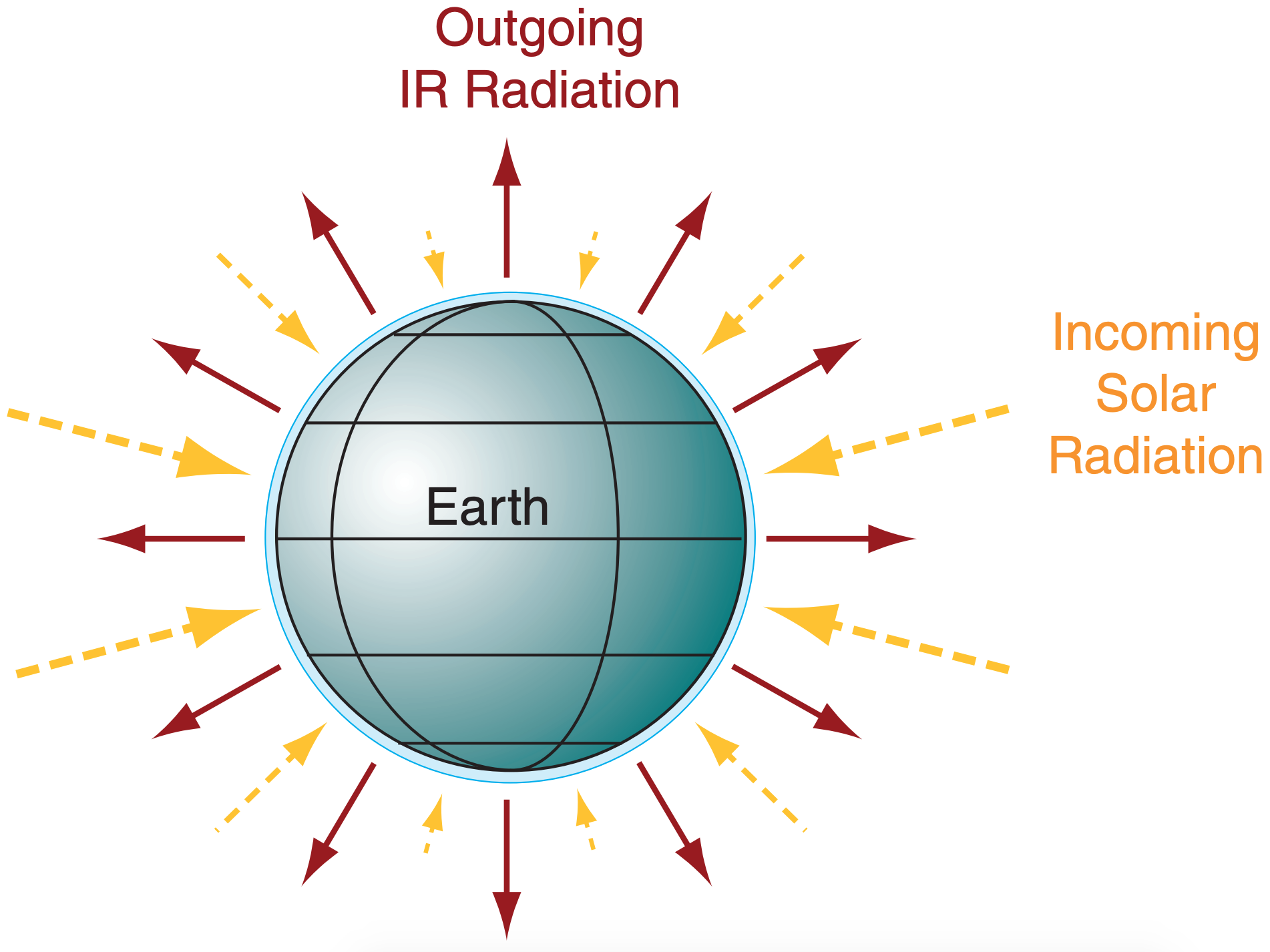
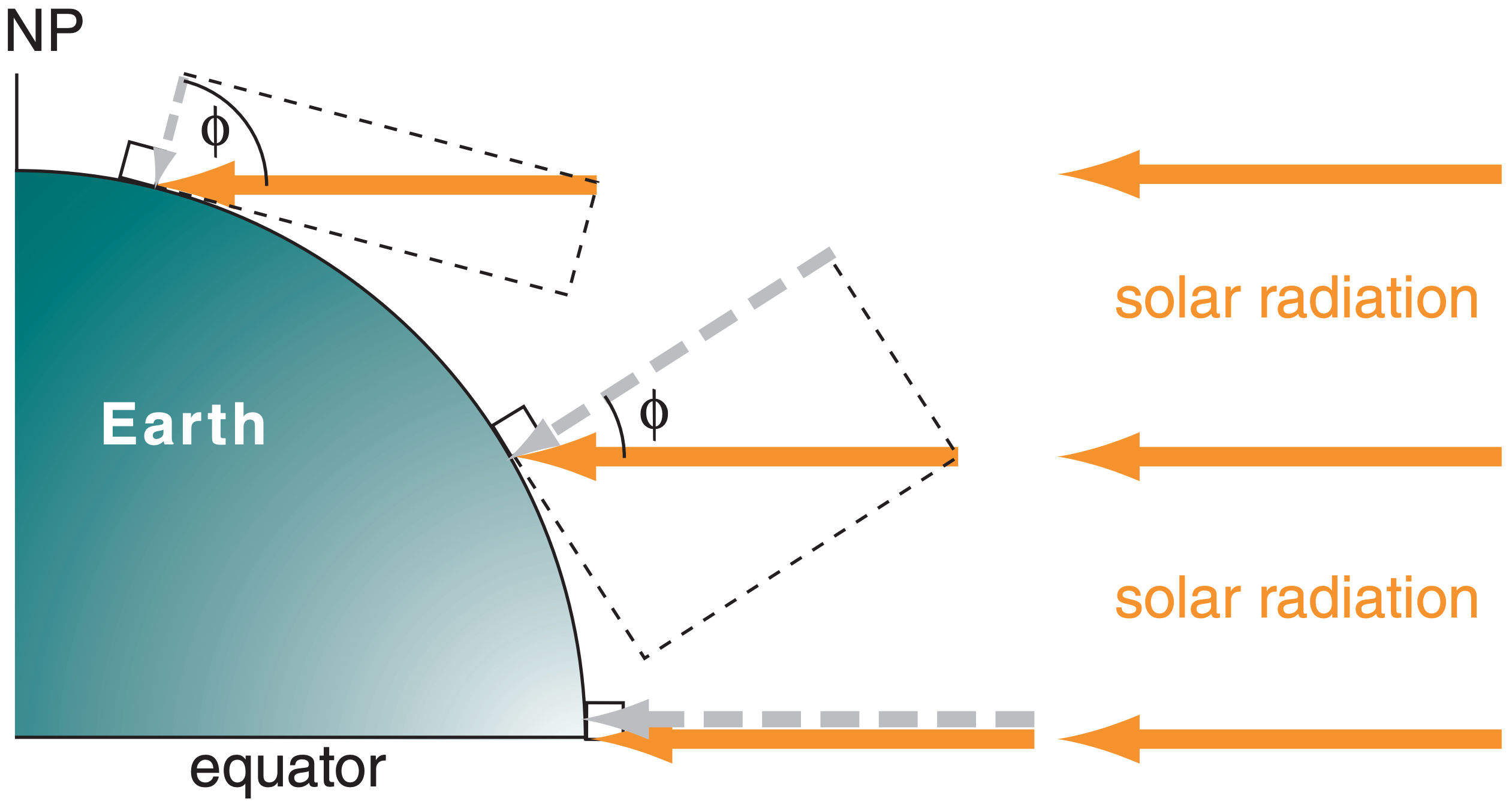
Recall from the Solar & Infrared Radiation chapter that the flux of solar radiation incident on the top of the atmosphere depends more or less on the cosine of the latitude, as shown in Fig. 11.7. The component of the incident ray of sunlight that is perpendicular to the Earth’s surface is small in polar regions, but larger toward the equator (grey dashed arrows in Figs. 11.6 and 11.7). The incoming energy adds heat to the Earth-atmosphere-ocean system.

Heat is lost due to infrared (IR) radiation emitted from the Earth-ocean-atmosphere system to space. Since all locations near the surface in the Earthocean-atmosphere system are relatively warm compared to absolute zero, the Stefan-Boltzmann law from the Solar & Infrared Radiation chapter tells us that the emission rates are also more or less uniform around the Earth. This is sketched by the solid red arrows in Fig. 11.6.

Thus, at low latitudes, more solar radiation is absorbed than leaves as IR, causing net warming. At high latitudes, the opposite is true: IR radiative losses exceed solar heating, causing net cooling. This differential heating drives the global circulation.

The general circulation can’t instantly eliminate all the global north-south temperature differences. What remains is a meridional temperature gradient — the focus of the next subsection.

11.3.1. North-South Temperature Gradient

Figure 11.8 Idealized variation of annual-average temperature (a) and meridional temperature gradient (b) with latitude, averaged around latitude belts (i.e., zonal averages). Solid curve represents Earth’s surface (= sea-level because the toy model neglects terrain) and dotted curve is for 15 km altitude above sea level.

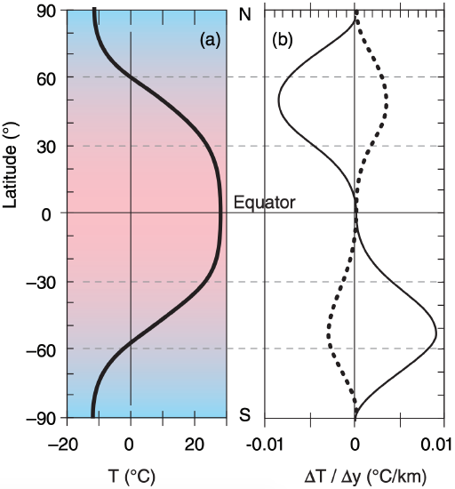
To create a first-order toy model, neglect monthly variations, monsoonal variations and mountains. Instead, focus on surface temperatures averaged around separate latitude belts and over one year. Those latitude belts near the equator are warmer, and those near the poles are colder (Fig. 11.8a). One equation that roughly approximates the variation of zonally-averaged surface temperature T with latitude ϕ is:

\(\ \begin{align} T \approx a+b \cdot\left[\cos ^{3} \phi \cdot\left(1+\frac{3}{2} \cdot \sin ^{2} \phi\right)\right]\tag{11.1}\end{align}\)

where a ≈ –12°C is an offset and b ≈ 40°C is a temperature difference between equator and pole.

The equation above applies only to the surface. At higher altitudes the north-south temperature difference is smaller, and even becomes negative in the stratosphere (i.e., warm over the poles and cold over the tropics). To account for this altitude variation, b cannot be a constant. Instead, use:

\(\ \begin{align} b \approx b_{1} \cdot\left(1-\frac{z}{z_{T}}\right)\tag{11.2}\end{align}\)

where average tropospheric depth is z_T ≈ 11 km, parameter b₁ = 40°C, and z is height above the surface.

A similarly crude but useful generalization of parameter a can be made so that it too changes with altitude z above sea level:

\(\ \begin{align} a \approx a_{1}-\gamma \cdot z\tag{11.3}\end{align}\)

where a₁ = –12°C and γ = 3.14 °C km^–1.

In Fig. 11.8a, the temperature curve looks like a flattened cosine wave. The flattened curve indicates somewhat uniformly warm temperatures between ±30° latitude, caused the strong mixing and heat transport by the Hadley circulations.

With uniform tropical temperatures, the remaining change to colder temperature is pushed to the mid-latitude belts. The slope of the Fig. 11.8a curve is plotted in Fig. 11.8b. This slope is the north-south (meridional) temperature gradient:

\(\ \begin{align} \frac{\Delta T}{\Delta y} \approx-b \cdot c \cdot \cos ^{2} \phi \cdot \sin ^{3} \phi\tag{11.4}\end{align}\)

where y is distance in the north-south direction, c = 1.18x10^–3 km^–1 is a constant valid at all heights, and b is given by eq. (11.2) which causes the gradient to change sign at higher altitudes (e.g., at z = 15 km).

Because the meridional temperature gradient results from the interplay of differential radiative heating and advection by the global circulation, let us now look at radiative forcings in more detail.

Sample Application

What is the value of annual zonal average temperature and meridional temperature gradient at 50°S latitude for the surface and for z = 15 km.

Find the Answer

Given: ϕ = –50°, (a) z = 0 (surface), and (b) z = 15 km

Find: T_sfc = ? °C, ∆T/∆y = ? °C km^–1

a) z = 0. Apply eq. (11.2): b = (40°C)·(1–0) = 40°C.

Apply eq. (11.3): a = (–12°C)–0°C = –12°C.

Apply eq. (11.1) :

\(\left.T_{o} \approx-12^{\circ} \mathrm{C}+\left(40^{\circ} \mathrm{C}\right) \cdot [\cos ^{3}\left(-50^{\circ}\right) \cdot\left(1+\frac{3}{2} \cdot \sin ^{2}\left(-50^{\circ}\right)\right)\right]=7.97^{\circ} \mathrm{C}\)

Apply eq. (11.4):

\(\frac{\Delta T}{\Delta y} \approx-\left(40^{\circ} \mathrm{C}\right) \cdot\left(1.18 \times 10^{-3}\right) \cdot \cos ^{2}\left(-50^{\circ}\right) \cdot \sin ^{3}\left(-50^{\circ}\right)=0.0087^{\circ} \mathrm{C} \mathrm{km}^{-1}\)

b) z = 15 km.

Apply eq. (11.2): b = (40°C)·[1–(15/11)] = –14.55°C.

Apply (11.3): a = (–12°C)–(3.14°C/km)·(15km) = –59.1°C.

Apply eq. (11.1) :

\(T_{15 k m} \approx-59.1^{\circ} \mathrm{C}-14.6^{\circ} \mathrm{C} \cdot\left[\cos ^{3}\left(-50^{\circ}\right) \cdot\left(1+\frac{3}{2} \cdot \sin ^{2}\left(-50^{\circ}\right)\right)\right]=-66.4^{\circ} \mathrm{C}\)

Apply eq. (11.4) at z = 15 km:

\(\frac{\Delta T}{\Delta y} \approx+\left(14.55^{\circ} \mathrm{C}\right) \cdot\left(1.18 \times 10^{-3}\right) \cdot \cos ^{2}\left(-50^{\circ}\right) \cdot \sin ^{3}\left(-50^{\circ}\right)=-0.0032^{\circ} \mathrm{C} \mathrm{km}^{-1}\)

Check: Phys. & units reasonable. Agrees with Fig. 11.8 for Southern Hemisphere.

Exposition: Cold at z = 15 km even though warm at z = 0. Gradient signs would be opposite in N. Hem.

11.3.2. Global Radiation Budgets

HIGHER MATH • Derivation of the NorthSouth Temperature Gradient

The goal is to find ∂T/∂y for the toy model.

a) First, expand the derivative: \(\ \begin{align} \frac{\partial T}{\partial y}=\frac{\partial T}{\partial \phi} \cdot \frac{\partial \phi}{\partial y}\tag{a}\end{align}\)

We will look at factors ∂T/∂ϕ and ∂ϕ/∂y separately:

b) Factor ∂ϕ/∂y describes the meridional gradient of latitude. Consider a circumference of the Earth that passes through both poles. The total latitude change around this circle is ∆ϕ = 2π radians. The total circumference of this circle is ∆y = 2πR for average Earth radius of R = 6371 km. Hence:

\(\ \begin{align} \frac{\partial \phi}{\partial y}=\frac{\Delta \phi}{\Delta y}=\frac{2 \pi}{2 \pi \cdot R}=\frac{1}{R}\tag{b}\end{align}\)

c) For factor ∂T/∂ϕ, start with eq. (11.1) for the toy model:

\(\ \begin{align} T \approx a+b \cdot\left[\cos ^{3} \phi \cdot\left(1+\frac{3}{2} \cdot \sin ^{2} \phi\right)\right]\tag{11.1}\end{align}\)

and take its derivative vs. latitude: \(\frac{\partial T}{\partial \phi}=b \cdot\left(\frac{3}{2}\right)\).

\(\left[(2 \sin \phi \cdot \cos \phi) \cos ^{3} \phi-3\left(\frac{2}{3}+\sin ^{2} \phi\right) \cos ^{2} \phi \cdot \sin \phi\right]\)

Next, take the common term (sinϕ · cos²ϕ) out of [ ]:

\(\frac{\partial T}{\partial \phi}=b\left(\frac{3}{2}\right) \sin \phi \cdot \cos ^{2} \phi \cdot\left[2 \cos ^{2} \phi-2-3 \sin ^{2} \phi\right]\)

Use the trig. identity: cos₂ϕ = 1 – sin2ϕ.

Hence: 2 cos²ϕ = 2 – 2 sin²ϕ . Substituting this in into the previous full-line equation gives:

\(\ \begin{align} \frac{\partial T}{\partial \phi}=b\left(\frac{3}{2}\right) \sin \phi \cdot \cos ^{2} \phi \cdot\left[-5 \sin ^{2} \phi\right]\tag{c}\end{align}\)

d) Plug equations (b) and (c) back into eq. (a):

\(\ \begin{align} \frac{\partial T}{\partial y}=-b \cdot\left(\frac{15}{2} \cdot \frac{1}{R}\right) \cdot \sin ^{3} \phi \cdot \cos ^{2} \phi\tag{d}\end{align}\)

Define:

\(c=\left(\frac{15}{2} \cdot \frac{1}{R}\right)=\left(\frac{15}{2} \cdot \frac{1}{6371 \mathrm{km}}\right)=1.177 \times 10^{-3} \mathrm{km}^{-1}\)

Thus, the final answer is:

\(\ \begin{align} \frac{\Delta T}{\Delta y}=\frac{\partial T}{\partial y}=-b \cdot c \cdot \sin ^{3} \phi \cdot \cos ^{2} \phi\tag{11.4}\end{align}\)

Check: Fig. 11.8 shows the curves that were calculated from eqs. (11.1) and (11.4). The fact that the sign and shape of the curve for ∆T/∆y is consistent with the curve for T(y) suggests the answer is reasonable.

Alert: Eqs. (11.4) and (11.1) are based on a highly idealized “toy model” of the real atmosphere. They were designed only to illustrate first-order effects.

11.3.2.1. Incoming Solar Radiation

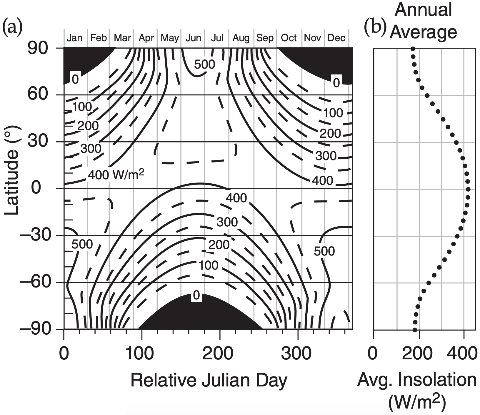
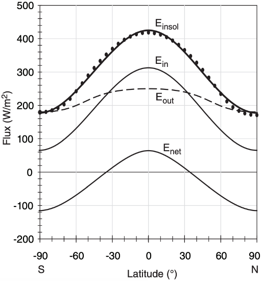
Because of the tilt of the Earth’s axis and the change of seasons, the actual flux of incoming solar radiation is not as simple as was sketched in Fig. 11.6. But this complication was already discussed in the Solar & Infrared Radiation chapter, where we saw an equation to calculate the incoming solar radiation (insolation) as a function of latitude and day. The resulting insolation figure is reproduced below (Fig. 11.9a).

If you take the spreadsheet data from the Solar & Infrared Radiation chapter that was used to make this figure, and average rows of data (i.e., average over all months for any one latitude), you can find the annual average insolation E_insol for each latitude (Fig. 11.9b). Insolation in polar regions is not small.

The curve in Fig. 11.9b is simple, and in the spirit of a toy model can be nicely approximated by:

\(\ \begin{align} E_{\text {insol}}=E_{o}+E_{1} \cdot \cos (2 \phi)\tag{11.5}\end{align}\)

where the empirical parameters are E_o = 298 W m^–2, E₁ = 123 W m^–2, and ϕ is latitude. This curve and the data points it approximates are plotted in Fig. 11.10.

But not all the radiation incident on the top of the atmosphere is absorbed by the Earth-ocean-atmosphere system. Some is reflected back into space from snow and ice on the surface, from the oceans, and from light-colored land. Some is reflected from cloud top. Some is scattered off of air molecules.

Figure 11.9 (a) Solar radiation (W m^–2) incident on the top of the atmosphere for different latitudes and months (copied from the Solar & Infrared Radiation chapter). The slight asymmetry about the equator is because Earth’s orbit is closer to the sun during S. Hemisphere summer. (b) Meridional variation of insolation, found by averaging the data from the left figure over all months for each separate latitude (i.e., averages for each row of data).

The amount of insolation that is NOT absorbed is surprisingly constant with latitude at about E₂ ≈ 110 W m^–2. Thus, the amount that IS absorbed is:

\(\ \begin{align} E_{i n}=E_{i n s o l}-E_{2}\tag{11.6}\end{align}\)

where E_in is the incoming flux (W m^–2) of solar radiation absorbed into the Earth-ocean-atmosphere system (Fig. 11.10). This absorbed radiation causes heating.

Figure 11.10 Data points are insolation vs. latitude from Fig. 11.9b. Eq. 11.5 approximates this insolation E_insol (thick black line). E_in is the solar radiation that is absorbed (thin solid line, from eq. 11.6). E_out is outgoing terrestrial (IR) radiation (dashed; from eq. 11.7). Net flux E_net = E_in – E_out. Positive Enet causes heating; negative causes cooling.

Sample Application

Estimate the annual average solar energy absorbed at the latitude of the Eiffel Tower in Paris, France.

Find the Answer

Given: ϕ = 48.8590° (at the Eiffel tower)

Find: E_in = ? W m^–2

Use eq. (11.5):

E_insol = (298 W m^–2) + (123 W m^–2)·cos(2 · 48.8590°)

= (298 W m^–2) – (16.5 W m^–2) = 281.5 W m^–2

Use eq. (11.6):

E_in = 281.5 W m^–2 – 110.0 W m^–2 = 171.5 W m^–2

Check: Units OK. Agrees with Fig. 11.10.

Exposition: The actual annual average E_in at the Eiffel Tower would probably differ from this zonal avg.

11.3.2.2. Outgoing Terrestrial Radiation

As you learned in the Satellites & Radar chapter, infrared radiation emission and absorption in the atmosphere are very complex. At some wavelengths the atmosphere is mostly transparent, while at others it is mostly opaque. Thus, some of the IR emissions to space are from the Earth’s surface, some from cloud top, and some from air at middle altitudes in the atmosphere.

In the spirit of a toy model, suppose that the net IR emissions are characteristic of the absolute temperature T_m near the middle of the troposphere (at about z_m = 5.5 km). Approximate the outbound flux of radiation E_out (averaged over a year and averaged around latitude belts) by the Stefan-Boltzmann law (see the Solar & Infrared Radiation chapter):

\(\ \begin{align} E_{o u t} \approx \varepsilon \cdot \sigma_{S B} \cdot T_{m}^{4}\tag{11.7}\end{align}\)

where the effective emissivity is ε ≈ 0.9 (see the Climate chapter), and the Stefan-Boltzmann constant is σ_SB = 5.67x10^–8 W·m^–2·K^–4. When you use z = z_m = 5.5 km in eqs. (11.1 - 11.3) to get T_m vs. latitude for use in eq. (11.7), the result is E_out vs. ϕ, as plotted in Fig. 11.10.

11.3.2.3. Net Radiation

For an air column over any square meter of the Earth’s surface, the radiative input minus output gives the net radiative flux:

\(\ \begin{align} E_{n e t}=E_{i n}-E_{o u t}\tag{11.8}\end{align}\)

which is plotted in Fig. 11.10 for our toy model.

Sample Application

What is E_net at the Eiffel Tower latitude?

Find the Answer

Given: ϕ = 48.8590°, z = 5.5 km, E_in = 171.5 W m^–2 from previous Sample Application

Find: E_net = ? W m^–2

Apply eq. (11.2): b = (40°C)·[ 1 – (5.5 km/11 km)] = 20°C

Apply eq.(11.3): a=(-12°C)–(3.14°C km^–1)·(5.5 km) = -29.27°C

Apply eq. (11.1): T_m = –18.73 °C = 254.5 K

Apply eq.(11.7): E_out=(0.9)·(5.67x10^–8W·m^–2·K^–4)·(254.5 K)⁴ = 213.8 W m^–2

Apply eq. (11.8): E_net = (171.5 W m^–2) – (213.8 W m^–2) = –42.3 W m^–2

Check: Units OK. Agrees with Fig. 11.10

Exposition: The net radiative heat loss at Paris latitude must be compensated by winds blowing heat in.

11.3.3. Radiative Forcing by Latitude Belt

Do you notice anything unreasonable about E_net in Fig. 11.10? It appears that the negative area under the curve is much greater than the positive area, which would cause the Earth to get colder and colder — an effect that is not observed.

Don’t despair. Eq. (11.8) is correct, but we must remember that the circumference [2π·R_Earth·cos(ϕ)] of a parallel (a constant latitude circle) is smaller near the poles than near the equator. ϕ is latitude and the average Earth radius R_Earth is 6371 km.

The solution is to multiply eqs. (11.6 - 11.8) by the circumference of a parallel. The result

\(\ \begin{align} E_{\phi}=2 \pi \cdot R_{E a r t h} \cdot \cos (\phi) \cdot E\tag{11.9}\end{align}\)

can be applied for E = E_in, or E = E_out, or E = E_net. This converts from E in units of W m^–2 to Eϕ in units of W m^–1, where the distance is north-south distance. You can interpret Eϕ as the power being transferred to/from a one-meter-wide sidewalk that encircles the Earth along a parallel.

Figure 11.11 Zonally-integrated radiative forcings for absorbed incoming solar radiation (solid line) and emitted net outgoing terrestrial (IR) radiation (dashed line). The surplus balances the deficit.

Figure 11.12 Net (incoming minus outgoing) zonally-integrated radiative forcings on the Earth. Surplus balances deficits. This differential heating imposed on the Earth must be compensated by heat transport by the global circulation; otherwise, the tropics would keep getting hotter and the polar regions colder.

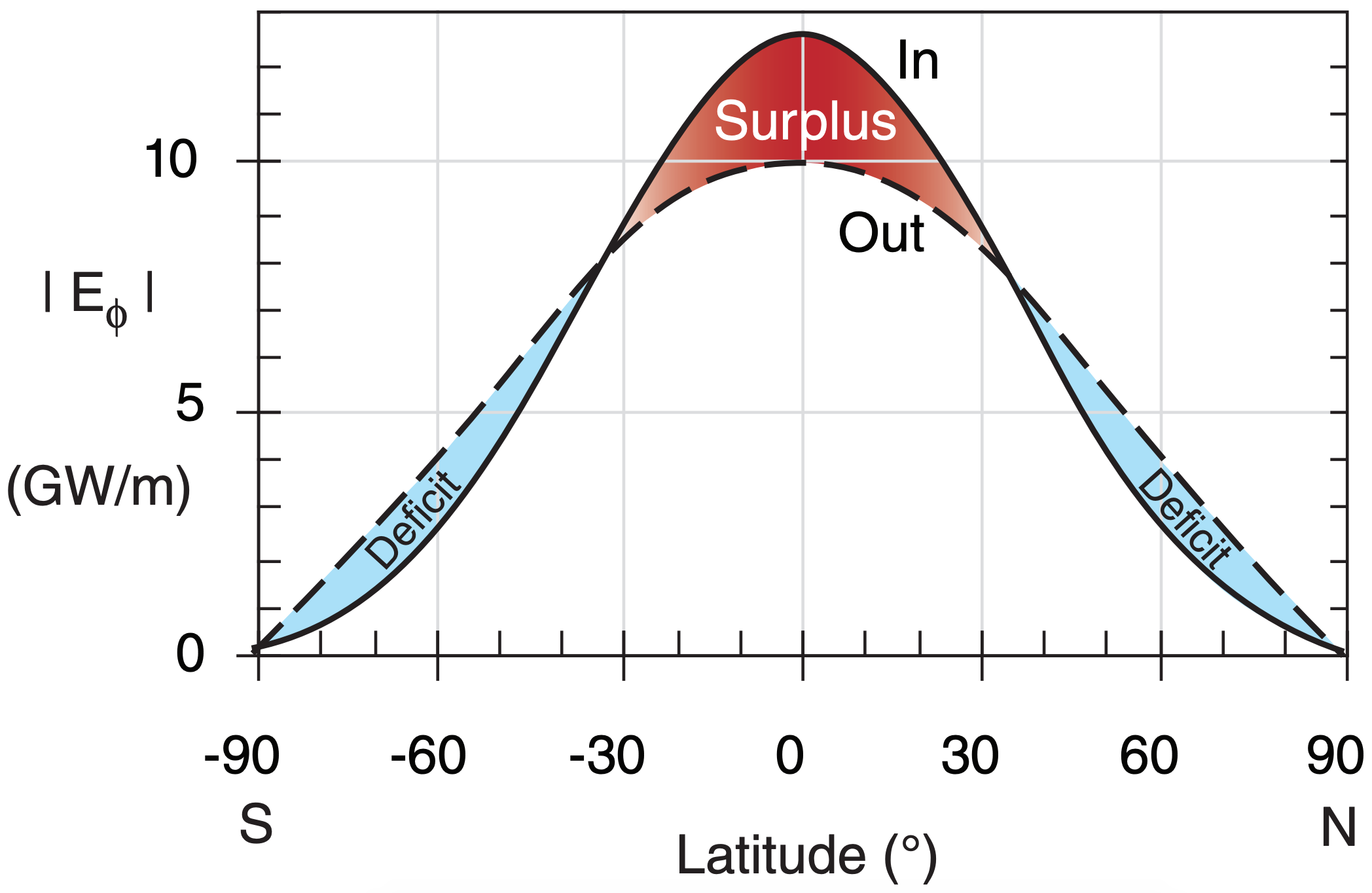
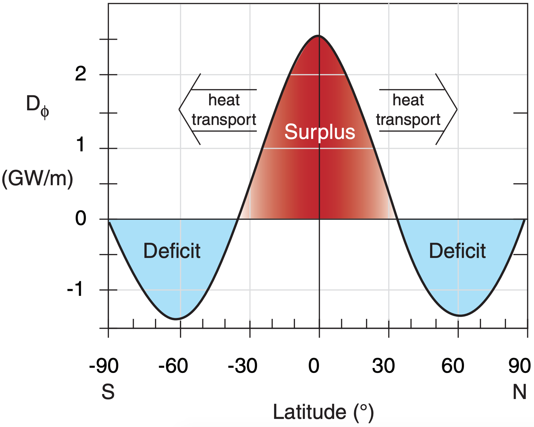
Figs. (11.11) and (11.12) show the resulting incoming, outgoing, and net radiative forcings vs. latitude. At most latitudes there is nonzero net radiation. We can define E_net as differential heating D_ϕ :

\(\ \begin{align} D_{\phi}=E_{\phi \text { net }}=E_{\phi \text { in }}-E_{\phi \text { out }}\tag{11.10}\end{align}\)

Our despair is now quelled, because the surplus and deficit areas in Figs. 11.11 and 11.12 are almost exactly equal in magnitude to each other. Hence, we anticipate that Earth’s climate should be relatively steady (neglecting global warming for now).

11.3.4. General Circulation Heat Transport

Nonetheless, the imbalance of net radiation between equator and poles in Fig. 11.12 drives atmospheric and oceanic circulations. These circulations act to undo the imbalance by removing the excess heat from the equator and depositing it near the poles (as per Le Chatelier’s Principle). First, we can use the radiative differential heating to find how much global-circulation heat transport is needed. Then, we can examine the actual heat transport by atmospheric and oceanic circulations.

11.3.4.1. The Amount of Transport Required

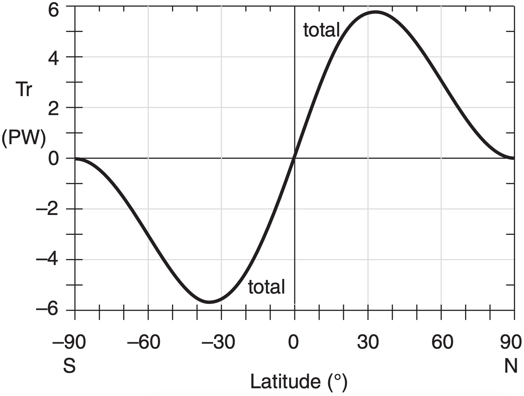
Meridional transport at each pole is zero, because the pole is a singularity where all meridians converge. If we sum D_ϕ from Fig. 11.12 over all latitude belts from the North Pole to any other latitude ϕ , we can find the total transport Tr required for the global circulation to compensate all the radiative imbalances north of that latitude:

\(\ \begin{align} \operatorname{Tr}(\phi)=\sum_{\phi_{0}=90^{\circ}}^{\phi}\left(-D_{\phi}\right) \cdot \Delta y\tag{11.11}\end{align}\)

where the width of any latitude belt is ∆y.

[Meridional distance ∆y is related to latitude change ∆ϕ by: ∆y(km) = (111 km/°) · ∆ϕ (°) .]

The resulting “needed transport” is shown in Fig. 11.13, based on the simple “toy model” temperature and radiation curves of the past few sections. The magnitude of this curve peaks at about 5.6 PW (1 petawatt equals 10¹⁵ W) at latitudes of about 35° North and South (positive Tr means northward transport).

Figure 11.13 Required heat transport Tr by the global circulation to compensate radiative differential heating, based on a simple “toy model”. Agrees very well with actual achieved transport in Fig. 11.14.

Figure 11.14 Meridional heat transports: Satellite-observed total (solid line) & ocean estimates (dotted). Atmospheric (dashed) is found as a residual. 1 PW = 1 petaWatt = 10¹⁵ W. [Data from K. E. Trenberth and J. M. Caron, 2001: “J. Climate”, 14, 3433-3443.]

11.3.4.2. Transport Achieved

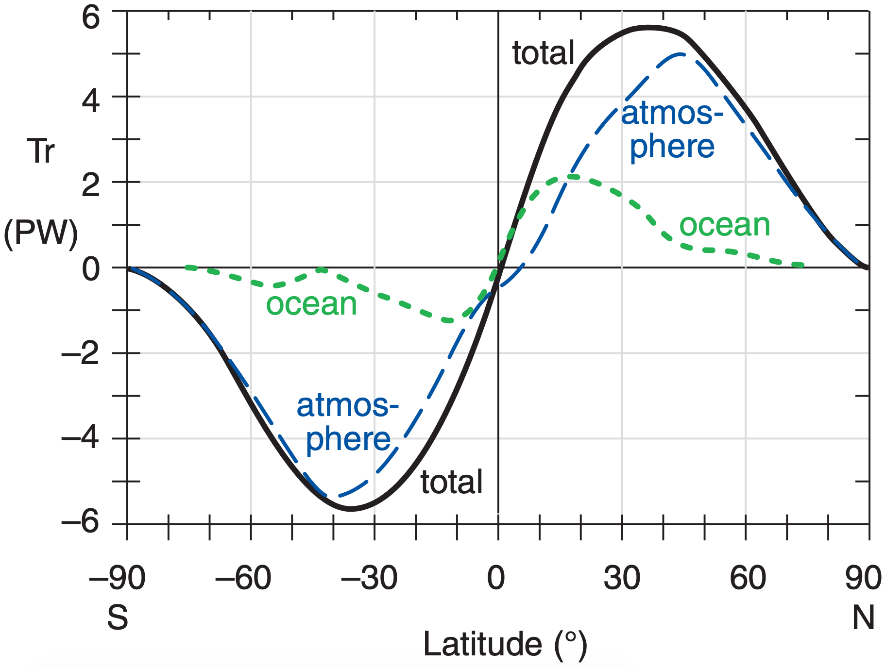
Satellite observations of radiation to and from the Earth, estimates of heat fluxes to/from the ocean based on satellite observations of sea-surface temperature, and in-situ measurements of the atmosphere provide some of the transport data needed. Numerical forecast models are then used to tie the observations together and fill in the missing pieces. The resulting estimate of heat transport achieved by the atmosphere and ocean is plotted in Fig. 11.14.

Ocean currents dominate the total heat transport only at latitudes 0 to 17°, and remain important up to latitudes of ± 40°. Asymmetry of the ocean curve across the equator is due to the different ocean basin shapes and currents. In the atmosphere, the Hadley circulation is a dominant contributor in the tropics and subtropics, while the Rossby waves dominate atmospheric transport at mid-latitudes.

Knowing that global circulations undo the heating imbalance raises another question. How does the differential heating in the atmosphere drive the winds in those circulations? That is the subject of the next three sections.

Sample Application

What total heat transports by the atmosphere and ocean circulations are needed at 50°N latitude to compensate for all the net radiative cooling between that latitude and the North Pole? The differential heating as a function of latitude is given in the following table (based on the toy model):

Lat (°)	Dϕ (GW m^–1)	Lat (°)	Dϕ (GW m^–1)
90	0	65	–1.380
85	–0.396	60	–1.403
80	–0.755	55	–1.331
75	–1.049	50	–1.164
70	–1.261	45	–0.905

Find the Answer

Given: ϕ = 50°N.

D_ϕ data in table above.

Find: Tr = ? PW

Use eq. (11.11). Use sidewalks (latitude belts) each of width ∆ϕ = 5°. Thus, ∆y (m) = (111,000 m/°) · (5°) = 555,000 m is the sidewalk width. If one sidewalk spans 85 - 90°, and the next spans 80 - 85° etc, then the values in the table above give D_ϕ along the edges of the sidewalk, not along the middle. A better approximation is to average the D_ϕ values from each edge to get a value representative of the whole sidewalk. Using a bit of algebra, this works out to:

Tr = – (555000 m)· [(0.5)·0.0 – 0.396 – 0.755 – 1.049 – 1.261 – 1.38 – 1.403 – 1.331 – (0.5)·1.164] (GW m^–1)

Tr = (555000 m)·[8.157 GW m^–1] = 4.527 PW

Check: Units OK (106 GW = 1 PW). Agrees with Fig. 11.14.

Exposition: This northward heat transport warms all latitudes north of 50°N, not just one sidewalk. The warming per sidewalk is ∆Tr/∆ϕ .