5.9: Finding tropopause Height and Mixed-Layer Depth
- Page ID
- 9922
5.8.1. Tropopause
Recall from Chapter 1 (Fig 1.10) that the standard-atmosphere temperature decreases with height within the troposphere, but is isothermal with height in the bottom part of the stratosphere. Isothermal layers are very strongly statically stable. The strong and deep statically stable layer in the stratosphere discourages vertical motion through it, which is why most of our weather (including thunderstorms and hurricanes) is trapped below it. The base of the stratospheric isothermal layer is the tropopause.
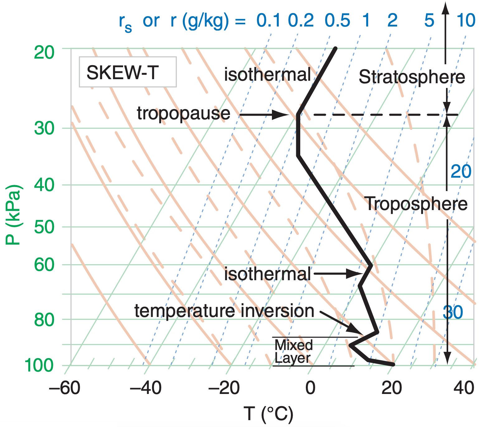
Real soundings are more complex than the simple standard atmosphere, and can have many different stable layers (and isothermal layers) at different heights (Figure 5.18). Nonetheless, if the radiosonde balloon rises high enough before bursting, then it often can enter the stratosphere. To locate the tropopause, we just need to look for the bottom of the very thick isothermal layer that is near a pressure altitude of 40 to 20 kPa.

Sample Application
What is the tropopause height (or pressure) in the sounding of Figure 5.18, and how is it identified?
Find the Answer
Given: the plotted sounding.
Find: PTrop = ? kPa
The base of the deep isothermal layer near the top of this sounding is at PTrop ≈ 28 kPa. The other isothermal and inversion layers are too low, and too thin.
Check: Sketch OK.
Exposition: The tropopause is lower near the poles and higher near the equator. It is lower in winter, higher in summer (see Table 6-1 in the Cloud chapter), but varies considerably from day to day.
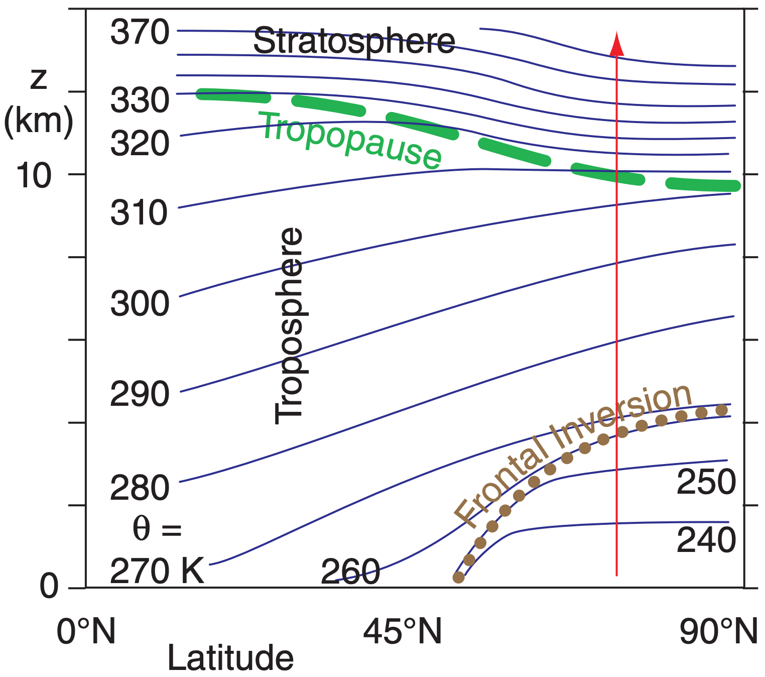
Strong static stability exists in regions where potential-temperature lines (isentropes) are vertically packed close together. The strongly stable stratosphere has tighter packing of isentropes than the less-stable troposphere, such as sketched in the idealized vertical cross section of Figure 5.19. Thus, you can locate the tropopause at the bottom of the region of tight isentrope packing, as sketched in Figure 5.19. [CAUTION: The tropopause usually does NOT follow any single isentrope.]

To illustrate the relationship between stability and isentrope spacing, suppose a rawinsonde (i.e., a helium-filled weather balloon) is released from near the ground and rises along the orange line in Figure 5.19. While it rises, it measures temperature and pressure of the surrounding environment, allowing one to calculate the vertical profile of potential temperature θ.
It starts in cold air near the ground, where the large spacing between isentropes shows that the static stability is weak near the ground. At about 4 km above the ground it passes through a frontal inversion, where static stability is stronger as shown by the close spacing of the two isentropes (θ = 260 & 270 K). Higher, in the mid troposphere, the larger spacing indicates weaker stability. Starting at about 10 km altitude the sonde enters a region of close spacing of isentropes, indicating that the sonde has entered the stratosphere. The bottom of this strongly stable region is the tropopause.
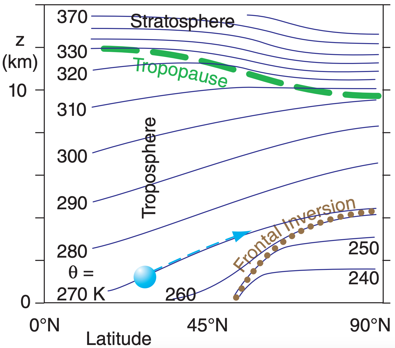
As air parcels advect (move) horizontally, they also tend to move vertically to stay on a surface of constant potential temperature (i.e., an isentropic surface), assuming no heat transfer to/from the parcel. The reason is buoyancy. For example, the parcel at 30°N illustrated in Figure 5.20 has a potential temperature of θ = 270 K, so it would try to stay on the 270 K isentrope (dark blue line in that figure).

If it were to stray slightly [above, below] that surface, it would be surrounded by air that has [warmer, cooler] potential temperature, causing a buoyant force that would tend to [lower, raise] the parcel back to the altitude of the 270 K isentrope. Isentropic analysis is a method of plotting weather variables on constant θ surfaces as a way to estimate dynamics under adiabatic conditions.
5.8.2. Mixed-Layer
When the sun heats the ground to be warmer than the adjacent air, or when cold air advects over warmer ground, some of the heat is conducted into the thin layer of air touching the ground (see the Thermodynamics chapter). This warm near-surface air wants to rise as bubbles or vertical plumes called thermals. You can sometimes see birds soaring in the updrafts of these thermals.
The thermals create vertical convective circulations that stir the bottom portion of the troposphere into a well-mixed layer. This convective mixed layer is evidence of nonlocal static instability in the boundary layer — the bottom 300 to 3000 m of the troposphere.
The mixed layer (ML) is usually capped by a statically stable layer or temperature inversion (where temperature increases with height), which prevents the thermals from rising through it and traps pollutants below it. Thus, the ML depth zi is important for air-quality studies.
To find zi from a sounding, use the nonlocal methods discussed earlier in this chapter. (1) Draw the measured sounding on a thermo diagram. (2) Estimate the temperature of the near-surface air parcel and plot it on the same diagram. (3) Lift this parcel adiabatically until it hits the environmental sounding, which defines zi (or Pi if using pressure as the vertical coordinate). θ vs. z thermo diagrams (see end of this chapter) are handy for ML studies.
A less accurate, but quick approach, is to look for the temperature inversion (or similar layer that is statically stable) that is near the ground, but not touching it. A temperature inversion is where T increases with height. The top of the mixed layer is usually somewhere within this temperature inversion. In Figure 5.18, the average height of the temperature inversion is about zi = 87 kPa. See the Boundary Layer and Air Pollution chapters for details.
Sample Application
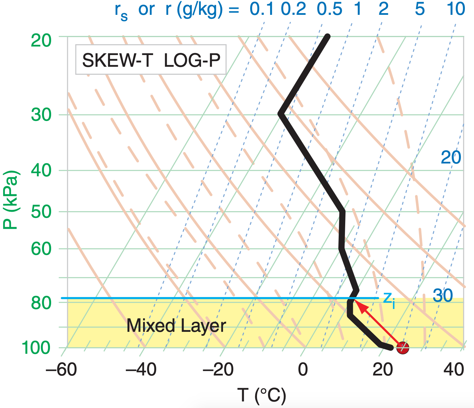
Plot the following sounding on a Skew-T diagram. If the ground heats an air parcel to the following state [P=100 kPa, T = 25°C], then find the pressure of the mixed-layer top. Sounding: [P (kPa), T (°C)] = [100,22] , [99,19] , [85,7] , [80,5] , [75,5] , [60,–5] , [50,–10] , [30,–40] , [20,–40] .
Find the Answer
Given: the data above.
Find: Pi (pressure in kPa at mixed-layer top zi ) See Skew-T below. Red dot and arrow represent the heated near-surface air parcel. Black line is the plotted environmental sounding.

From the diagram, Pi ≈ 78 kPa.
Check: Sketch agrees with larger thermo diagrams.
Exposition: The yellow-shaded region is nonlocally unstable. It is the turbulent mixed layer.
The nonlocal approach is not new. Thunderstorm forecasters usually use the whole sounding, and consider air parcels rising from the surface to the top of the storm to estimate the potential severity of storms. They don’t focus on only the local lapse rate in the mid troposphere to estimate thunderstorm intensity.
“Lapse rate” (subadiabatic, adiabatic, superadiabatic) is not synonymous with “static stability” (stable, neutral, unstable). If the purpose of a stability definition is to determine whether flow becomes turbulent, then you must consider nonlocal effects within the whole sounding.


