5.4: More on the Skew-T

Last updated
Save as PDF

Page ID: 9556

\( \newcommand{\vecs}[1]{\overset { \scriptstyle \rightharpoonup} {\mathbf{#1}} } \) \( \newcommand{\vecd}[1]{\overset{-\!-\!\rightharpoonup}{\vphantom{a}\smash {#1}}} \)\(\newcommand{\id}{\mathrm{id}}\) \( \newcommand{\Span}{\mathrm{span}}\) \( \newcommand{\kernel}{\mathrm{null}\,}\) \( \newcommand{\range}{\mathrm{range}\,}\) \( \newcommand{\RealPart}{\mathrm{Re}}\) \( \newcommand{\ImaginaryPart}{\mathrm{Im}}\) \( \newcommand{\Argument}{\mathrm{Arg}}\) \( \newcommand{\norm}[1]{\| #1 \|}\) \( \newcommand{\inner}[2]{\langle #1, #2 \rangle}\) \( \newcommand{\Span}{\mathrm{span}}\) \(\newcommand{\id}{\mathrm{id}}\) \( \newcommand{\Span}{\mathrm{span}}\) \( \newcommand{\kernel}{\mathrm{null}\,}\) \( \newcommand{\range}{\mathrm{range}\,}\) \( \newcommand{\RealPart}{\mathrm{Re}}\) \( \newcommand{\ImaginaryPart}{\mathrm{Im}}\) \( \newcommand{\Argument}{\mathrm{Arg}}\) \( \newcommand{\norm}[1]{\| #1 \|}\) \( \newcommand{\inner}[2]{\langle #1, #2 \rangle}\) \( \newcommand{\Span}{\mathrm{span}}\)\(\newcommand{\AA}{\unicode[.8,0]{x212B}}\)

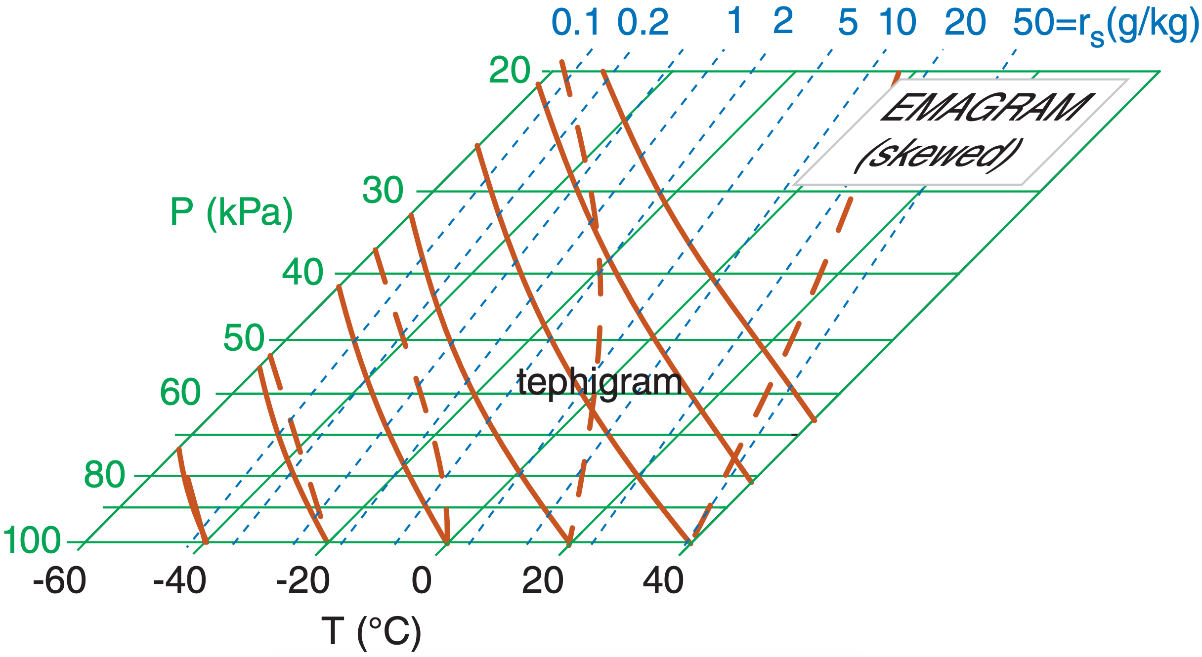
Because of the popularity of the Skew-T, we dissect it in Figure 5.4, to aid in its interpretation. Tephigram users should find this equally useful, because the only noticeable difference is that the isobars are slightly curved, and increase in slope higher in the tephigram.

The Skew-T diagram is trivial to create, once you have already created an Emagram. The easiest way is to start with a graphic image of an Emagram, and skew it into a parallelogram (Figure 5.5) using a graphics or drawing program.

Screen Shot 2020-02-12 at 11.17.58 AM.png — Figure 5.5 A Skew-T is nothing more than a skewed Emagram.

It is equally simple to draw a Skew-T with a spreadsheet program, especially if you start with the numbers you already calculated to create an Emagram. Let X (°C) be the abscissa of a Cartesian graph, and Y (dimensionless) be the ordinate. Let K be the skewness factor, which is arbitrary. A value of K = 35°C gives a nice skewness (such that the isotherms and adiabats are nearly perpendicular), but you can pick any skewness you want.

The coordinates for any point on the graph are:

\(\ \begin{align} Y=\ln \left(\frac{P_{o}}{P}\right)\tag{5.1a}\end{align}\)

\(\ \begin{align} X=T+K \cdot Y\tag{5.1b}\end{align}\)

To draw isotherms, set T to the isotherm value, and find a set of X values corresponding to different heights Y. Plot this one line as an isotherm. For the other isotherms, repeat for other values of T. [Hint: it is convenient to set the spreadsheet program to draw a logarithmic vertical axis with the max and min reversed. If you do this, then use P, not Y, as your vertical coordinate. But you still must use Y in the equation above to find X.]

For the isohumes, dry adiabats, and moist adiabats, use the temperatures you found for the Emagram as the input temperatures in the equation above. For example, the θ = 20°C adiabat has the following temperatures as a function of pressure (recall Thermo Diagrams-Part 1, in the Thermodynamics chapter), from which the corresponding values of X can be found.

P(kPa)= 100 , 80 , 60 , 40 , 20

T(°C) = 20 , 1.9 , –19.8, –47.5 , –88

X = 20 , 9.7 , –1.9 , –15.4 , –31.7

Sample Application

Create a Skew-T diagram with one isotherm (T = 20°C), one dry adiabat (θ = 20°C), one moist adiabat (θ_w = 20°C), and one isohume (r = 5 g/kg). Use as input the temperatures from the Emagram (as calculated in earlier chapters). Use K = 35°C, and P_o = 100 kPa.

Find the Answer

Given: The table of Emagram numbers below. Use eq. (5.1) in a spreadsheet to find X and Y.

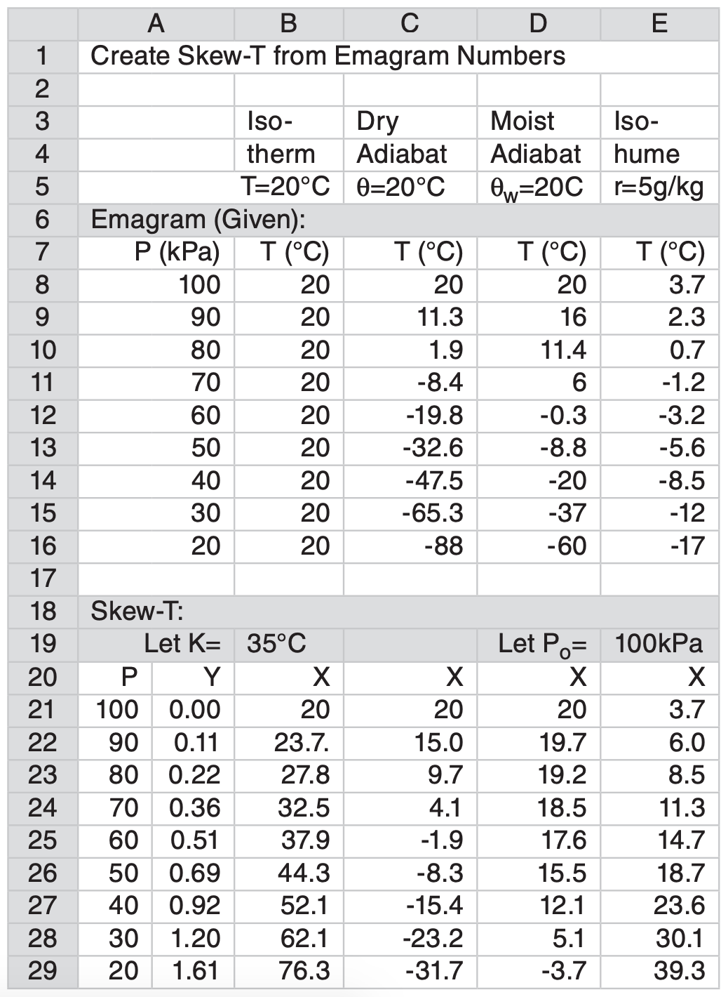
Screen Shot 2020-02-12 at 11.26.59 AM.png

Using the spreadsheet to plot the result gives:

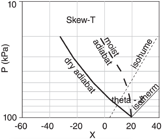
Screen Shot 2020-02-12 at 11.28.23 AM.png

Check: Sketch reasonable. Matches Figure 5.4e.

Exposition: Experiment with different values of K starting with K = 0°C, and see how the graph changes from an Emagram to a Skew-T.