Geosciences LibreTexts

5.3: 5.2. Types of Thermo Diagrams

  • Page ID
    9555
  • \( \newcommand{\vecs}[1]{\overset { \scriptstyle \rightharpoonup} {\mathbf{#1}} } \)

    \( \newcommand{\vecd}[1]{\overset{-\!-\!\rightharpoonup}{\vphantom{a}\smash {#1}}} \)

    \( \newcommand{\id}{\mathrm{id}}\) \( \newcommand{\Span}{\mathrm{span}}\)

    ( \newcommand{\kernel}{\mathrm{null}\,}\) \( \newcommand{\range}{\mathrm{range}\,}\)

    \( \newcommand{\RealPart}{\mathrm{Re}}\) \( \newcommand{\ImaginaryPart}{\mathrm{Im}}\)

    \( \newcommand{\Argument}{\mathrm{Arg}}\) \( \newcommand{\norm}[1]{\| #1 \|}\)

    \( \newcommand{\inner}[2]{\langle #1, #2 \rangle}\)

    \( \newcommand{\Span}{\mathrm{span}}\)

    \( \newcommand{\id}{\mathrm{id}}\)

    \( \newcommand{\Span}{\mathrm{span}}\)

    \( \newcommand{\kernel}{\mathrm{null}\,}\)

    \( \newcommand{\range}{\mathrm{range}\,}\)

    \( \newcommand{\RealPart}{\mathrm{Re}}\)

    \( \newcommand{\ImaginaryPart}{\mathrm{Im}}\)

    \( \newcommand{\Argument}{\mathrm{Arg}}\)

    \( \newcommand{\norm}[1]{\| #1 \|}\)

    \( \newcommand{\inner}[2]{\langle #1, #2 \rangle}\)

    \( \newcommand{\Span}{\mathrm{span}}\) \( \newcommand{\AA}{\unicode[.8,0]{x212B}}\)

    \( \newcommand{\vectorA}[1]{\vec{#1}}      % arrow\)

    \( \newcommand{\vectorAt}[1]{\vec{\text{#1}}}      % arrow\)

    \( \newcommand{\vectorB}[1]{\overset { \scriptstyle \rightharpoonup} {\mathbf{#1}} } \)

    \( \newcommand{\vectorC}[1]{\textbf{#1}} \)

    \( \newcommand{\vectorD}[1]{\overrightarrow{#1}} \)

    \( \newcommand{\vectorDt}[1]{\overrightarrow{\text{#1}}} \)

    \( \newcommand{\vectE}[1]{\overset{-\!-\!\rightharpoonup}{\vphantom{a}\smash{\mathbf {#1}}}} \)

    \( \newcommand{\vecs}[1]{\overset { \scriptstyle \rightharpoonup} {\mathbf{#1}} } \)

    \( \newcommand{\vecd}[1]{\overset{-\!-\!\rightharpoonup}{\vphantom{a}\smash {#1}}} \)

    \(\newcommand{\avec}{\mathbf a}\) \(\newcommand{\bvec}{\mathbf b}\) \(\newcommand{\cvec}{\mathbf c}\) \(\newcommand{\dvec}{\mathbf d}\) \(\newcommand{\dtil}{\widetilde{\mathbf d}}\) \(\newcommand{\evec}{\mathbf e}\) \(\newcommand{\fvec}{\mathbf f}\) \(\newcommand{\nvec}{\mathbf n}\) \(\newcommand{\pvec}{\mathbf p}\) \(\newcommand{\qvec}{\mathbf q}\) \(\newcommand{\svec}{\mathbf s}\) \(\newcommand{\tvec}{\mathbf t}\) \(\newcommand{\uvec}{\mathbf u}\) \(\newcommand{\vvec}{\mathbf v}\) \(\newcommand{\wvec}{\mathbf w}\) \(\newcommand{\xvec}{\mathbf x}\) \(\newcommand{\yvec}{\mathbf y}\) \(\newcommand{\zvec}{\mathbf z}\) \(\newcommand{\rvec}{\mathbf r}\) \(\newcommand{\mvec}{\mathbf m}\) \(\newcommand{\zerovec}{\mathbf 0}\) \(\newcommand{\onevec}{\mathbf 1}\) \(\newcommand{\real}{\mathbb R}\) \(\newcommand{\twovec}[2]{\left[\begin{array}{r}#1 \\ #2 \end{array}\right]}\) \(\newcommand{\ctwovec}[2]{\left[\begin{array}{c}#1 \\ #2 \end{array}\right]}\) \(\newcommand{\threevec}[3]{\left[\begin{array}{r}#1 \\ #2 \\ #3 \end{array}\right]}\) \(\newcommand{\cthreevec}[3]{\left[\begin{array}{c}#1 \\ #2 \\ #3 \end{array}\right]}\) \(\newcommand{\fourvec}[4]{\left[\begin{array}{r}#1 \\ #2 \\ #3 \\ #4 \end{array}\right]}\) \(\newcommand{\cfourvec}[4]{\left[\begin{array}{c}#1 \\ #2 \\ #3 \\ #4 \end{array}\right]}\) \(\newcommand{\fivevec}[5]{\left[\begin{array}{r}#1 \\ #2 \\ #3 \\ #4 \\ #5 \\ \end{array}\right]}\) \(\newcommand{\cfivevec}[5]{\left[\begin{array}{c}#1 \\ #2 \\ #3 \\ #4 \\ #5 \\ \end{array}\right]}\) \(\newcommand{\mattwo}[4]{\left[\begin{array}{rr}#1 \amp #2 \\ #3 \amp #4 \\ \end{array}\right]}\) \(\newcommand{\laspan}[1]{\text{Span}\{#1\}}\) \(\newcommand{\bcal}{\cal B}\) \(\newcommand{\ccal}{\cal C}\) \(\newcommand{\scal}{\cal S}\) \(\newcommand{\wcal}{\cal W}\) \(\newcommand{\ecal}{\cal E}\) \(\newcommand{\coords}[2]{\left\{#1\right\}_{#2}}\) \(\newcommand{\gray}[1]{\color{gray}{#1}}\) \(\newcommand{\lgray}[1]{\color{lightgray}{#1}}\) \(\newcommand{\rank}{\operatorname{rank}}\) \(\newcommand{\row}{\text{Row}}\) \(\newcommand{\col}{\text{Col}}\) \(\renewcommand{\row}{\text{Row}}\) \(\newcommand{\nul}{\text{Nul}}\) \(\newcommand{\var}{\text{Var}}\) \(\newcommand{\corr}{\text{corr}}\) \(\newcommand{\len}[1]{\left|#1\right|}\) \(\newcommand{\bbar}{\overline{\bvec}}\) \(\newcommand{\bhat}{\widehat{\bvec}}\) \(\newcommand{\bperp}{\bvec^\perp}\) \(\newcommand{\xhat}{\widehat{\xvec}}\) \(\newcommand{\vhat}{\widehat{\vvec}}\) \(\newcommand{\uhat}{\widehat{\uvec}}\) \(\newcommand{\what}{\widehat{\wvec}}\) \(\newcommand{\Sighat}{\widehat{\Sigma}}\) \(\newcommand{\lt}{<}\) \(\newcommand{\gt}{>}\) \(\newcommand{\amp}{&}\) \(\definecolor{fillinmathshade}{gray}{0.9}\)

    5.2.1. Emagram

    “Emagram” is a contraction for “Energy-perunit-mass diagram.” This semi-log diagram (Figure 5.3a) has temperature (T) along the abscissa, and pressure (P) decreasing logarithmically upward along the ordinate. The isotherms and isobars are straight lines that are perpendicular to each other, and form the orthogonal basis for this diagram.

    Dry adiabats (θ) are nearly-straight, diagonal lines slanted up towards the left, and curve slightly concave upward. Moist adiabats (θw) curve concave downward, but become parallel to the dry adiabats at cold temperatures and high altitudes. Isohumes (r) are nearly-straight, nearly-vertical lines (with a slight tilt upward to the left).

    Height contours (on the large Emagram at the end of this chapter) are approximate, and are provided as a rough guide to users. These contours are nearly horizontal (tilting downward slightly to the right) and nearly straight (slightly concave upward). They are often not drawn in thermo diagrams, and indeed are not shown in Figs. 5.1 and 5.3.

    5.2.2. Stüve & Pseudoadiabatic Diagrams

    The Stüve diagram (Figure 5.3b) has T along the abscissa, and pressure decreasing upward along the ordinate according to (P/Po)ℜd/Cpd , where ℜd/Cpd = 0.28571 (dimensionless) and Po = 100 kPa. Stüve diagrams look virtually identical to Emagrams, except that the dry adiabats are perfectly straight. These dry adiabats converge to a point at P = 0 kPa and T = 0 K, which is usually well off of the upper left corner of the graph.

    Any thermo diagram can be computed using the pseudoadiabatic assumption for the moist adiabats. However, the particular diagram that is known as a “Pseudoadiabatic Diagram” is often a Stüve plot.

    5.2.3. Skew-T Log-P Diagram

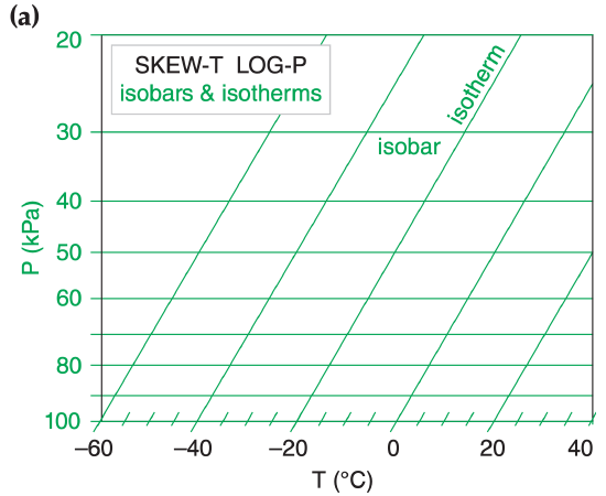
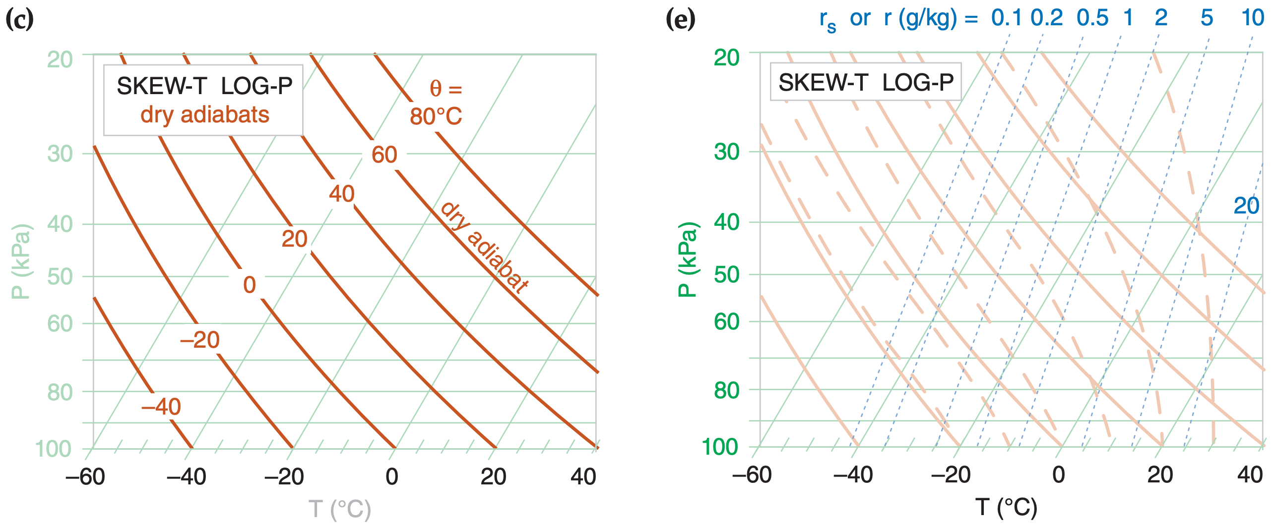
    Figure 5.3c is a Skew-T. Although T is labeled linearly along the abscissa, the isotherms are parallel, straight, diagonal lines tilting upward to the right. The Skew-T gets its name because the isotherms are not vertical, but skewed. Pressure decreases logarithmically upward along the ordinate, and the isobars are parallel, horizontal, straight lines.

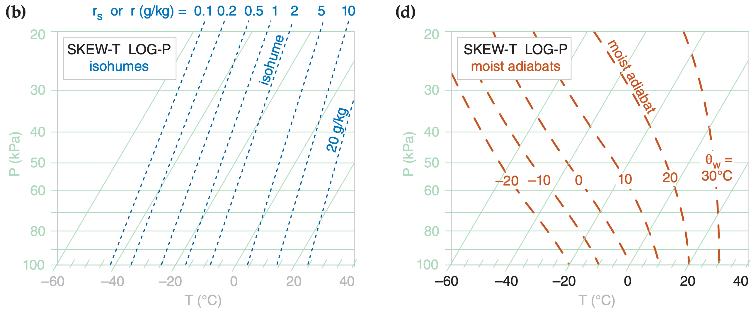
    Dry adiabats are diagonal lines slanted up towards the left, with a pronounced curve concave upward. Moist adiabats are more sharply curved concave left near the bottom of the diagram, changing to less curved, concave to the right, as they merge into the dry adiabats at higher altitudes and colder temperatures. Isohumes are almost straight lines, tilting upward to the right.

    This diagram is designed so that the isotherms and dry adiabats are nearly (but not perfectly) perpendicular to each other.

    5.2.4. Tephigram

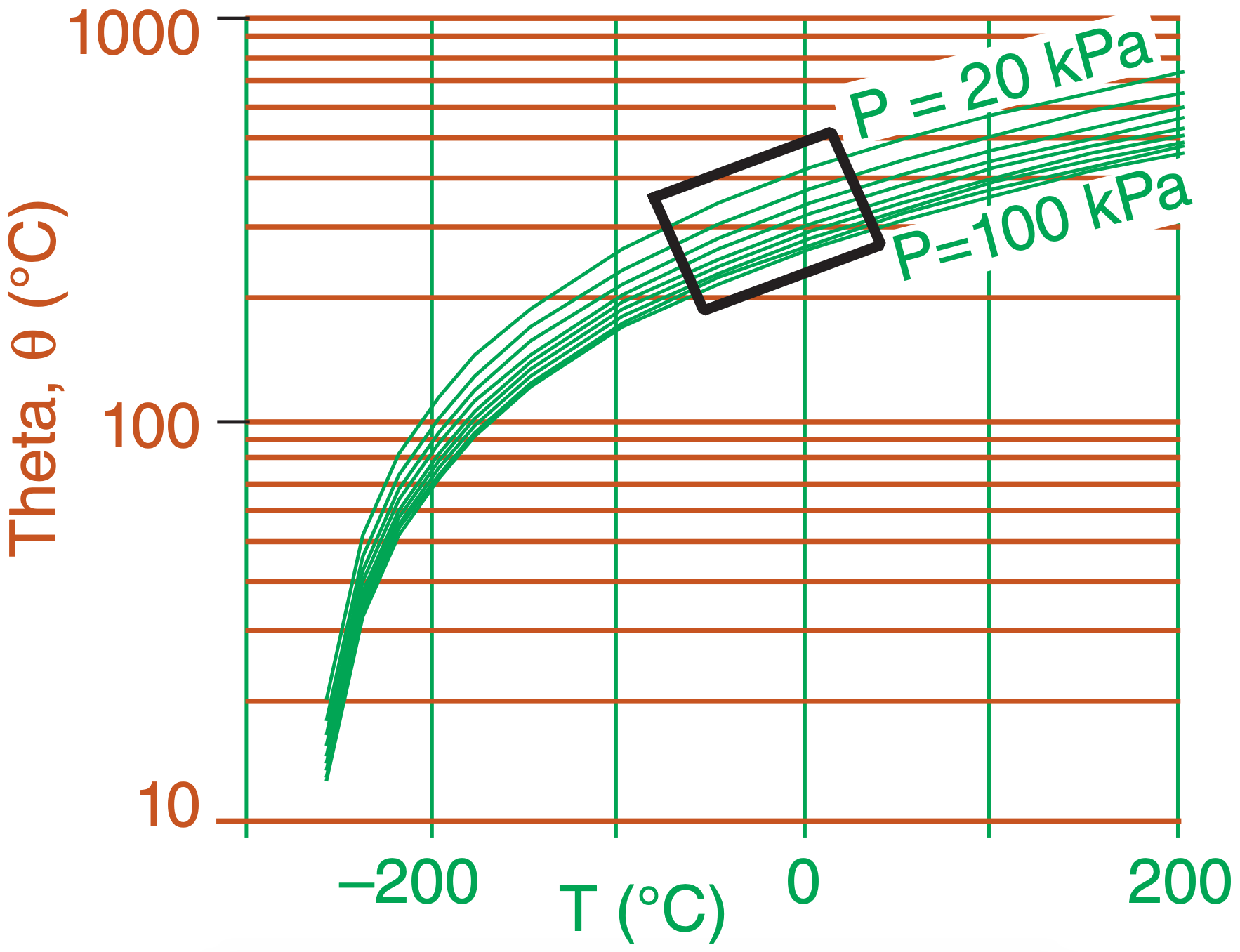
    The name Tephigram is a contraction of Tee-Phi Diagram. The logarithm of potential temperature θ physically represents the entropy (ϕ = Greek letter Phi) change, and is plotted along the ordinate of Figure 5.2. Temperature T is along the abscissa. Thus, it is a temperature-entropy diagram, or T-ϕ diagram. Isobars are curved green lines in Figure 5.2.

    The range of meteorological interest is shown with the bold rectangle in this figure. When this region is enlarged and tilted horizontally, the result is the tephigram as plotted in Figure 5.3d.
    Screen Shot 2020-02-12 at 11.04.25 AM.png
    Figure 5.2 Rectangle shows portion of thermo diagram used for tephigram.

    The tephigram looks similar to the Skew-T, with isotherms as straight diagonal lines tilting upward to the right. Dry adiabats are perfectly straight diagonal lines tilting upward left, and are exactly perpendicular to the isotherms. Moist adiabats have strong curvature concave left, and become parallel to the dry adiabats at cold temperatures and high altitudes. Isobars are gently curved (concave down) nearly-horizontal lines. Isohumes are nearly straight diagonal lines tilting upward right.

    5.2.5. Theta-Height (θ-z) Diagrams

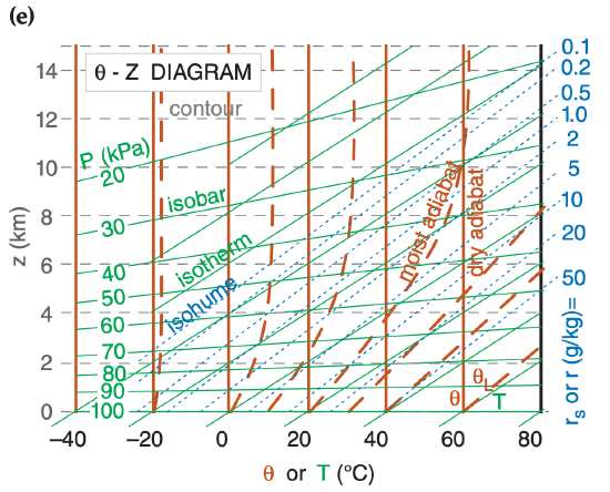
    The orthogonal basis for this diagram are heights (z) plotted along the ordinate and potential temperature (θ) along the abscissa (Figure 5.3e). Moist adiabats curve to the right of the dry adiabats, but become parallel to the dry adiabats at high altitudes and cold temperatures. Heights are accurate in this diagram, but the isobars are only approximate. Isohumes tilt steeply upward to the right. This diagram is used extensively in boundary-layer meteorology.
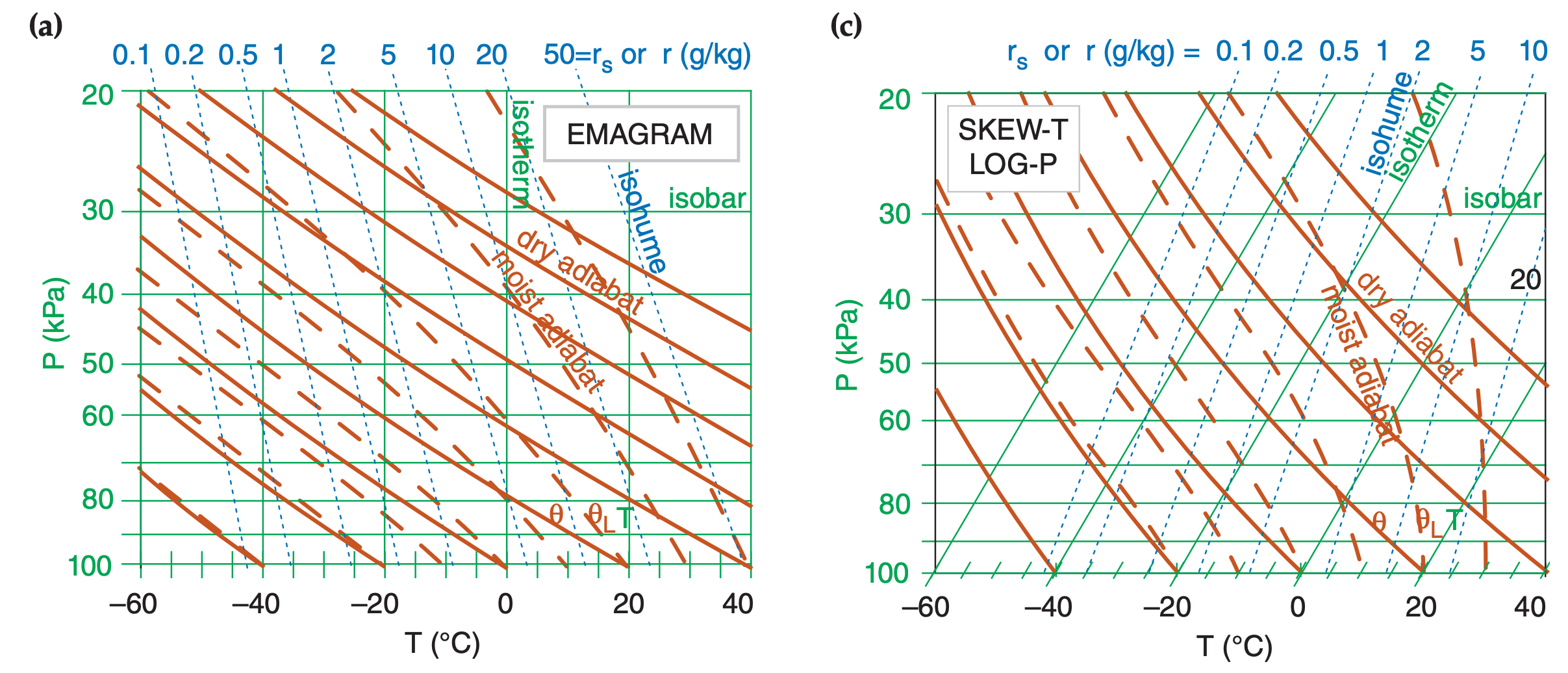
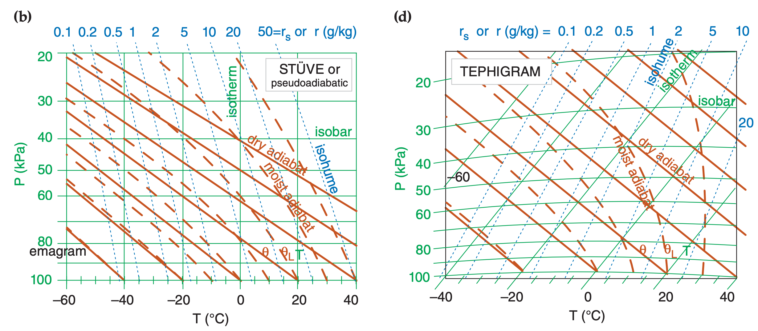
    Figure 5.3 Catalog of thermodynamic diagrams. In all diagrams, thick dark-orange lines represent processes, and thin lines (green or blue) represent state. Thick solid dark-orange lines are dry adiabats, and thick dashed dark-orange are moist adiabats. Solid thin green horizontal or nearly-horizontal lines are pressure, and solid thin green vertical or diagonal straight lines are temperature. Isohumes are thin dotted blue lines. In addition, the θ-z diagram has height contours (z) as thin horizontal dashed grey lines.

    Screen Shot 2020-02-12 at 11.07.31 AM.png

    Screen Shot 2020-02-12 at 11.08.10 AM.pngScreen Shot 2020-02-12 at 11.08.29 AM.png

    Screen Shot 2020-02-12 at 11.11.53 AM.pngScreen Shot 2020-02-12 at 11.12.37 AM.pngScreen Shot 2020-02-12 at 11.13.20 AM.png
    Figure 5.4 (a)-(d) Components of a Skew-T diagram, drawn to the same scale so they can be superimposed as a learning aid. The state of the air: (a) isobars and isotherms; (b) isohumes as thin dotted lines. Processes: (c) dry adiabats; (d) moist adiabats. (e) Full Skew-T Log-P, shaded lighter to make it easier to write on. The “Skew-T Log-P” diagram is often called a “Skew-T” for short.

    This page titled 5.3: 5.2. Types of Thermo Diagrams is shared under a CC BY-NC-SA 4.0 license and was authored, remixed, and/or curated by Roland Stull via source content that was edited to the style and standards of the LibreTexts platform.

    • Was this article helpful?