
11.4: Pressure Profiles
- Page ID
- 9599

If something you cannot measure contributes to things you can measure, then you can estimate the unknown as the residual (i.e., difference) from all the knowns. This is a valid scientific approach. It was used in Fig. 11.14 to estimate the atmospheric portion of global heat transport.
CAUTION: When using this approach, your residual not only includes the desired signal, but it also includes the sums of all the errors from the items you measured. These errors can easily accumulate to cause a “noise” that is larger than the signal you are trying to estimate. For this reason, error estimation and error propagation (see Appendix A) should always be done when using the method of residuals.
The following fundamental concepts can help you understand how the global circulation works:
- non-hydrostatic pressure couplets caused by horizontal winds and vertical buoyancy,
- hydrostatic thermal circulations,
- geostrophic adjustment, and
- the thermal wind.
The first two concepts are discussed in this section. The last two are discussed in subsequent sections.
11.4.1. Non-hydrostatic Pressure Couplets
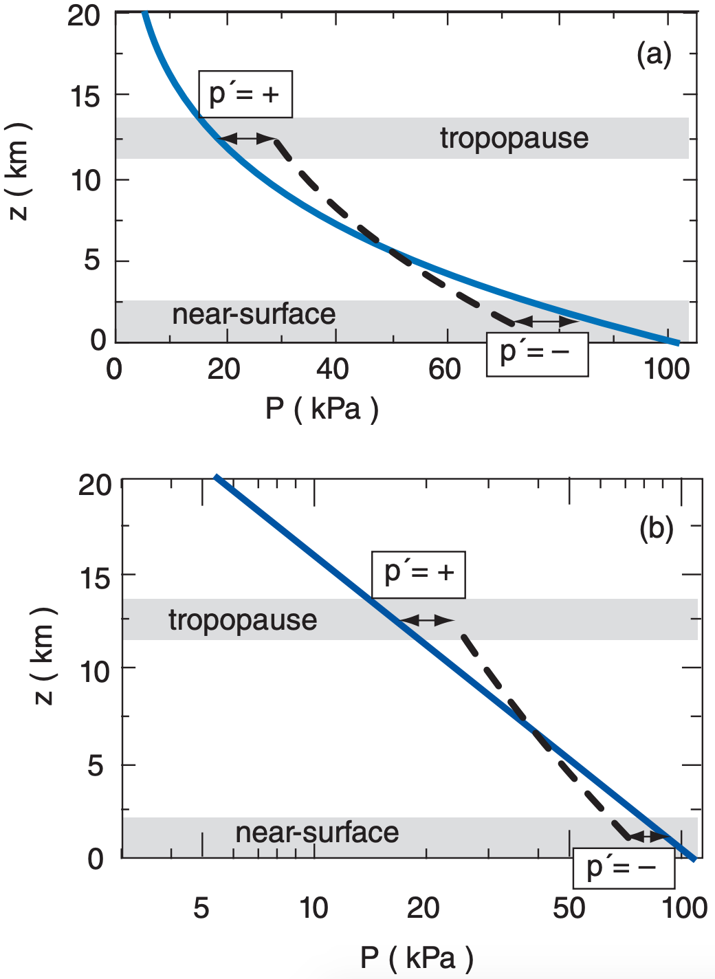
Consider a background reference environment with no vertical acceleration (i.e., hydrostatic). Namely, the pressure-decrease with height causes an upward pressure-gradient force that exactly balances the downward pull of gravity, causing zero net vertical force on the air (see Fig. 1.12 and eq. 1.25).
Next, suppose that immersed in this environment is a column of air that might experience a different pressure decrease (Fig. 11.15); i.e., non-hydrostatic pressures. At any height, let p’ = Pcolumn – Phydrostatic be the deviation of the actual pressure in the column from the theoretical hydrostatic pressure in the environment. Often a positive p’ in one part of the atmospheric column is associated with negative p’ elsewhere. Taken together, the positive and negative p’s form a pressure couplet.
Non-hydrostatic p’ profiles are often associated with non-hydrostatic vertical motions through Newton’s second law. These non-hydrostatic motions can be driven by horizontal convergence and divergence, or by buoyancy (a vertical force). These two effects create opposite pressure couplets, even though both can be associated with upward motion, as explained next.
11.4.1.1. Horizontal Convergence/Divergence
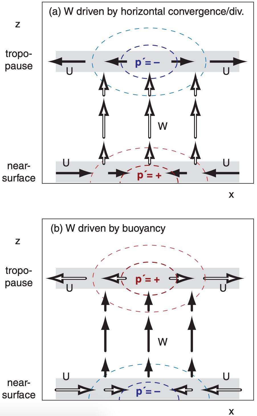
If external forcings cause air near the ground to converge horizontally, then air molecules accumulate. As density ρ increases according to eq. (10.60), the ideal gas law tells us that p’ will also become positive (Fig. 11.16a). Non-zero p’ implies that a pressure gradient exists, which will drive winds.
Positive p’ does two things: it (1) decelerates the air that was converging horizontally, and (2) accelerates air vertically in the column. Thus, the pressure perturbation causes mass continuity (horizontal inflow near the ground balances vertical outflow).
Similarly, an externally imposed horizontal divergence at the top of the troposphere would lower the air density and cause negative p’, which would also accelerate air in the column upward. Hence, we expect upward motion (W = positive) to be driven by a p’ couplet, as shown in Fig. 11.16a.
11.4.1.2. Buoyant Forcings
For a different scenario, suppose air in a column is positively buoyant, such as in a thunderstorm where water-vapor condensation releases lots of latent heat. This vertical buoyant force creates upward motion (i.e., warm air rises, as in Fig. 11.16b).
As air in the thunderstorm column moves away from the ground, it removes air molecules and lowers the density and the pressure; hence, p’ is negative near the ground. This suction under the updraft causes air near the ground to horizontally converge, thereby conserving mass.
Conversely, at the top of the troposphere where the thunderstorm updraft encounters the even warmer environmental air in the stratosphere, the upward motion rapidly decelerates, causing air molecules to accumulate, making p’ positive. This pressure perturbation drives air to diverge horizontally near the tropopause, causing the outflow in the anvil-shaped tops of thunderstorms.
The resulting pressure-perturbation p’ couplet in Fig. 11.16b is opposite that in Fig. 11.16a, yet both are associated with upward vertical motion. The reason for this pressure-couplet difference is the difference in driving mechanism: imposed horizontal convergence/divergence vs. imposed vertical buoyancy.
Similar arguments can be made for downward motions. For either upward or downward motions, the pressure couplets that form depend on the type of forcing. We will use this process to help explain the pressure patterns at the top and bottom of the troposphere.
11.4.2. Hydrostatic Thermal Circulations
Cold columns of air tend to have high surface pressures, while warm columns have low surface pressures. Figs. 11.17 illustrate how this happens.
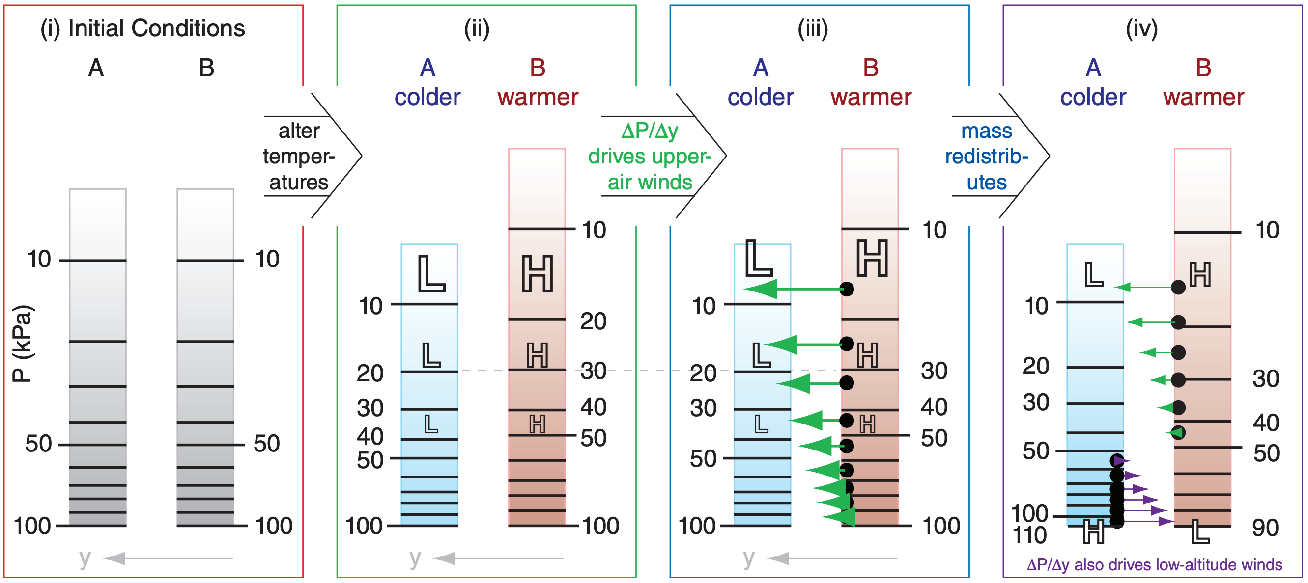
Consider initial conditions (Fig. 11.17i) of two equal columns of air at the same temperature and with the same number of air molecules in each column. Since pressure is related to the mass of air above, this means that both columns A and B have the same initial pressure (100 kPa) at the surface.
Next, suppose that some process heats one column relative to the other (Fig. 11.17ii). Perhaps condensation in a thunderstorm cloud causes latent heating of column B, or infrared radiation cools column A. After both columns have finished expanding or contracting due to the temperature change, they will reach new hydrostatic equilibria for their respective temperatures.
The hypsometric equation (see Chapter 1) says that pressure decreases more rapidly with height in cold air than in warm air. Thus, although both columns have the same surface pressure because they contain the same number of molecules, the higher you go above the surface, the greater is the pressure difference between warm and cold air. In Fig. 11.17ii, the printed size of the “H” and “L” indicate the relative magnitudes of the high- and low-pressure perturbations p’.
The horizontal pressure gradient ∆P/∆y aloft between the warm and cold air columns drives horizontal winds from high toward low pressure (Fig. 11.17iii). Since winds are the movement of air molecules, this means that molecules leave the regions of high pressure-perturbation and accumulate in the regions of low. Namely, they leave the warm column, and move into the cold column.
Since there are now more molecules (i.e., more mass) in the cold column, it means that the surface pressure must be greater (H) in the cold column (Fig. 11.17iv). Similarly, mass lost from the warm column results in lower (L) surface pressure. This is called a thermal low.
A result (Fig. 11.17iv) is that, near the surface, high pressure in the cold air drives winds toward the low pressure in warm air. Aloft, high pressureperturbation in the warm air drives winds towards low pressure-perturbation in the cold air. The resulting thermal circulation causes each column to gain as many air molecules as they lose; hence, they are in mass equilibrium.
This equilibrium circulation also transports heat. Air from the warm air column mixes into the cold column, and vice versa. This intermixing reduces the temperature contrast between the two columns, causing the corresponding equilibrium circulations to weaken. Continued destabilization (more latent heating or radiative cooling) would be needed to maintain the circulation.
The circulations and mass exchange described above can be realized at the equator. At other latitudes, the exchange of mass is often slower (near the surface) or incomplete (aloft) because Coriolis force turns the winds to some angle away from the pressure-gradient direction. This added complication, due to geostrophic wind and geostrophic adjustment, is described next.