6.6: Cloud Sizes

Last updated
Save as PDF

Page ID: 9566

\( \newcommand{\vecs}[1]{\overset { \scriptstyle \rightharpoonup} {\mathbf{#1}} } \) \( \newcommand{\vecd}[1]{\overset{-\!-\!\rightharpoonup}{\vphantom{a}\smash {#1}}} \)\(\newcommand{\id}{\mathrm{id}}\) \( \newcommand{\Span}{\mathrm{span}}\) \( \newcommand{\kernel}{\mathrm{null}\,}\) \( \newcommand{\range}{\mathrm{range}\,}\) \( \newcommand{\RealPart}{\mathrm{Re}}\) \( \newcommand{\ImaginaryPart}{\mathrm{Im}}\) \( \newcommand{\Argument}{\mathrm{Arg}}\) \( \newcommand{\norm}[1]{\| #1 \|}\) \( \newcommand{\inner}[2]{\langle #1, #2 \rangle}\) \( \newcommand{\Span}{\mathrm{span}}\) \(\newcommand{\id}{\mathrm{id}}\) \( \newcommand{\Span}{\mathrm{span}}\) \( \newcommand{\kernel}{\mathrm{null}\,}\) \( \newcommand{\range}{\mathrm{range}\,}\) \( \newcommand{\RealPart}{\mathrm{Re}}\) \( \newcommand{\ImaginaryPart}{\mathrm{Im}}\) \( \newcommand{\Argument}{\mathrm{Arg}}\) \( \newcommand{\norm}[1]{\| #1 \|}\) \( \newcommand{\inner}[2]{\langle #1, #2 \rangle}\) \( \newcommand{\Span}{\mathrm{span}}\)\(\newcommand{\AA}{\unicode[.8,0]{x212B}}\)

Cumuliform clouds typically have diameters roughly equal to their depths, as mentioned previously. For example, a fair weather cumulus cloud typically averages about 1 km in size, while a thunderstorm might be 10 km.

Not all clouds are created equal. At any given time the sky contains a spectrum of cloud sizes that has a lognormal distribution (Figure 6.10, eq. 6.6)

\[\ \begin{align} f(X)=\frac{\Delta X}{\sqrt{2 \pi} \cdot X \cdot S_{X}} \cdot \exp \left[-0.5 \cdot\left(\frac{\ln \left(X / L_{X}\right)}{S_{X}}\right)^{2}\right]\end{align} \label{6.6}\]

where \(X\) is the cloud diameter or depth, \(∆X\) is a small range of cloud sizes, \(f(X)\) is the fraction of clouds of sizes between \(X–0.5∆X\) and \(X+0.5∆X\), \(L_x\) is a location parameter, and \(S_x\) is a dimensionless spread parameter. These parameters vary widely in time and location.

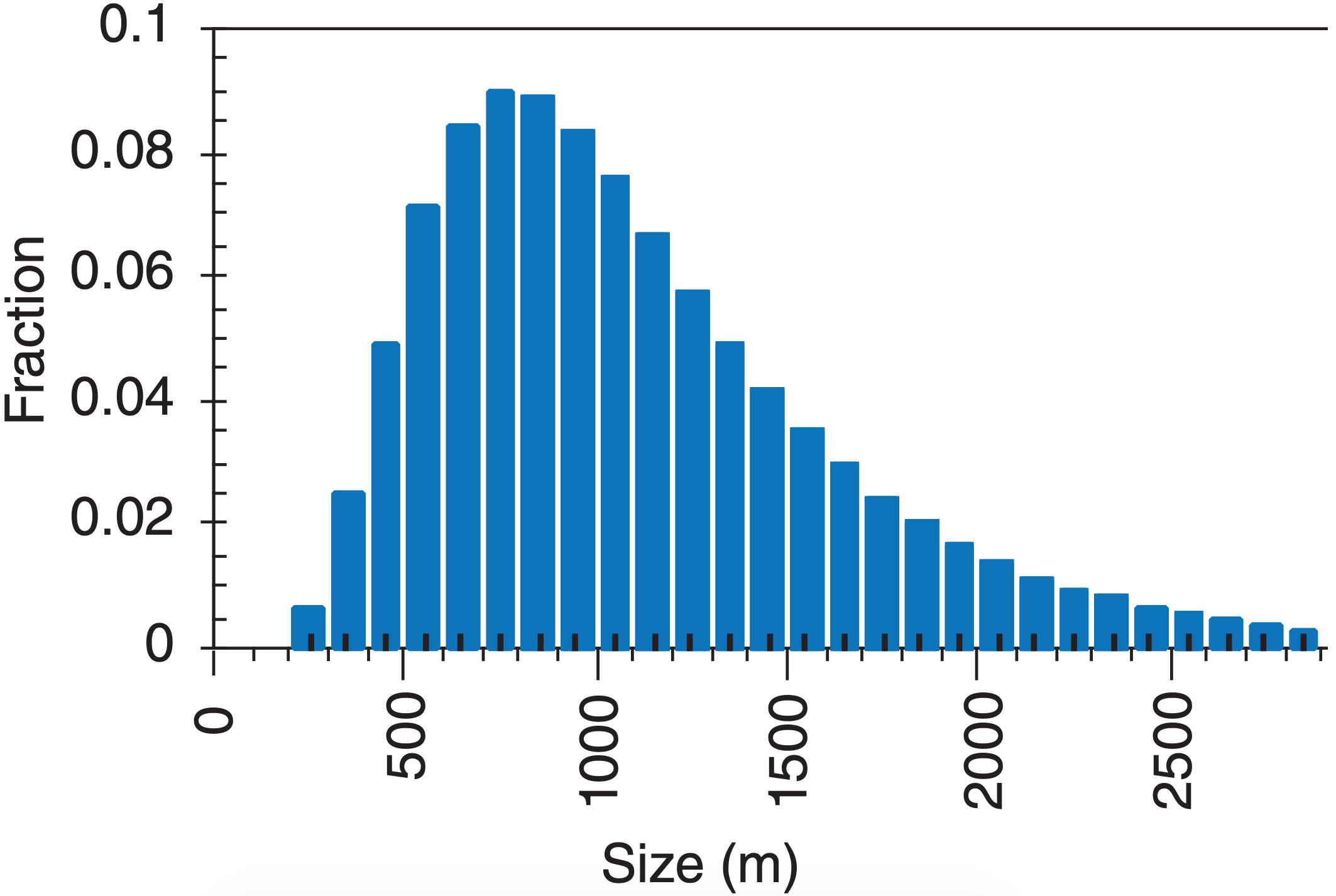
Screen Shot 2020-02-16 at 2.36.26 AM.png — Figure 6.10: Lognormal distribution of cloud sizes.

According to this distribution, there are many clouds of nearly the same size, but there also are a few clouds of much larger size. This causes a skewed distribution with a long tail to the right (Figure 6.10).

Sample Application

Use a spreadsheet to find and plot the fraction of clouds ranging from X = 50 to 4950 m width, given ∆X = 100 m, S_X =0.5, and L_X = 1000 m.

Find the Answer

Given: ∆X = 100 m, S_X =0.5, L_X = 1000 m.

Find: f(X)= ?

Solve eq. (6.6) on a spreadsheet. The result is:

X (m)	f(X)
50	2.558x10^–8
150	0.0004
250	0.0068
350	0.0252
450	0.0495
550	0.0710 etc.
Sum of all	f = 0.999

Check: Units OK. Physics almost OK, but the sum of all f should equal 1.0, representing 100% of the clouds. The reason for the error is that we should have considered clouds even larger than 4950 m, because of the tail on the right of the distribution. Also smaller ∆X would help.

Exposition: Although the dominant cloud width is about 800 m for this example, the long tail on the right of the distribution shows that there are also a small number of large-diameter clouds.