13.5: Ascent

You can also use updraft speed to estimate cyclone strength and the associated clouds. For the case-study cyclone, Fig. 13.25 shows upward motion near the middle of the troposphere (at 50 kPa).

Recall from classical physics that the definition of vertical motion is W = ∆z/∆t, for altitude z and time t. Because each altitude has an associated pressure, define a new type of vertical velocity in terms of pressure. This is called omega (ω):

\(\ \begin{align} \omega=\frac{\Delta P}{\Delta t}\tag{13.13}\end{align}\)

Omega has units of Pa s^–1.

You can use the hydrostatic equation to relate W and ω:

\(\ \begin{align} \omega=-\rho \cdot|g| \cdot W\tag{13.14}\end{align}\)

for gravitational acceleration magnitude |g| = 9.8 m·s^–2 and air density ρ. The negative sign in eq. (13.14) implies that updrafts (positive W) are associated with negative ω. As an example, if your weather map shows ω = –0.68 Pa s^–1 on the 50 kPa surface, then the equation above can be rearranged to give W = 0.1 m s^–1, where an mid-tropospheric density of ρ ≈ 0.69 kg·m^–3 was used.

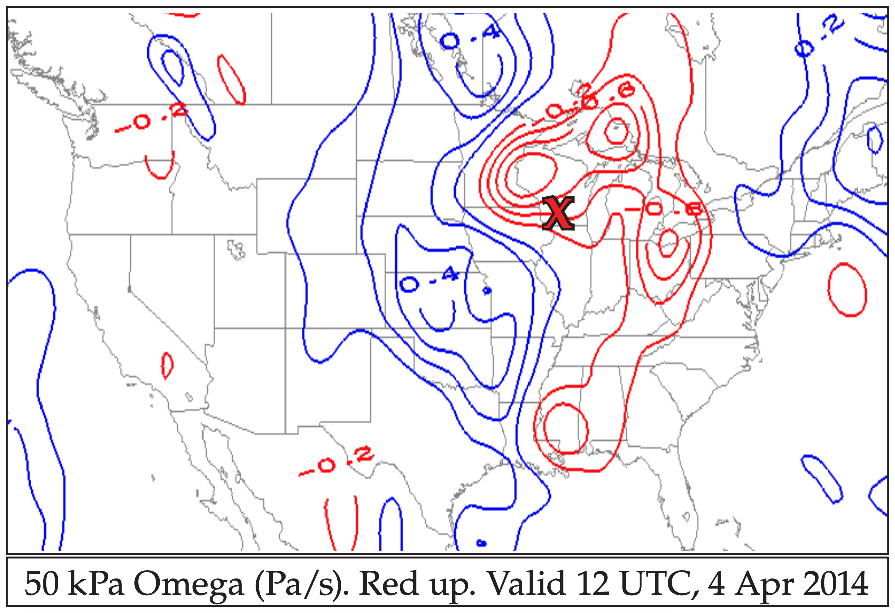
Use either W or ω to represent vertical motion. Numerical weather forecasts usually output the vertical velocity as ω. For example, Fig. 13.28 shows upward motion (ω) near the middle of the troposphere (at 50 kPa).

Figure 13.28 Vertical velocity (omega) in pressure coordinates, for the casestudy cyclone. Negative omega (colored red on this map) corresponds to updrafts.

The following three methods will be employed to study ascent: the continuity equation, the omega equation, and Q-vectors. Near the tropopause, horizontal divergence of jet-stream winds can force midtropospheric ascent in order to conserve air mass as given by the continuity equation. The almost-geostrophic (quasi-geostrophic) nature of lower-tropospheric winds allows you to estimate ascent at 50 kPa using thermal-wind and vorticity principles in the omega equation. Q-vectors consider ageostrophic motions that help maintain quasi-geostrophic flow. These methods are just different ways of looking at the same processes, and they often give similar results.

Sample Application

At an elevation of 5 km MSL, suppose (a) a thunderstorm has an updraft velocity of 40 m s^–1, and (b) the subsidence velocity in the middle of an anticyclone is –0.01 m s^–1. Find the corresponding omega values.

Find the Answer

Given: (a) W = 40 m s^–1. (b) W = – 0.01 m s^–1. z = 5 km.

Find: ω = ? kPa s^–1 for (a) and (b).

To estimate air density, use the standard atmosphere table from Chapter 1: ρ = 0.7361 kg m^–3 at z = 5 km.

Next, use eq. (13.14) to solve for the omega values:

(a) ω = –(0.7361 kg m^–3)·(9.8 m s^–2)·(40 m s^–1)

= –288.55 (kg·m^–1·s^–2)/s = –288.55 Pa s^–1

= –0.29 kPa/s

(b) ω = –(0.7361 kg m^–3)·(9.8 m s^–2)·(–0.01 m s^–1)

= 0.0721 (kg·m^–1·s^–2)/s = 0.0721 Pa s^–1

= 7.21x10^–5 kPa s^–1

Check: Units and sign are reasonable.

Exposition: CAUTION. Remember that the sign of omega is opposite that of vertical velocity, because as height increases in the atmosphere, the pressure decreases. As a quick rule of thumb, near the surface where air density is greater, omega (in kPa s–1) has magnitude of roughly a hundredth of W (in m s–1), with opposite sign.

13.5.1. Continuity Effects

Horizontal divergence (D = ∆U/∆x + ∆V/∆y) is where more air leaves a volume than enters, horizontally. This can occur at locations where jet-stream wind speed (M_out) exiting a volume is greater than entrance speeds (M_in).

Conservation of air mass requires that the number of air molecules in a volume, such as the light blue region sketched in Fig. 13.29, must remain nearly constant (neglecting compressibility). Namely, volume inflow must balance volume outflow of air.

Figure 13.29 For air in the top half of the troposphere (shaded light blue), if air leaves faster (M_out) than enters (M_in) horizontally, then continuity requires that this upper-level horizontal divergence be balanced by ascent W_mid in the mid troposphere.

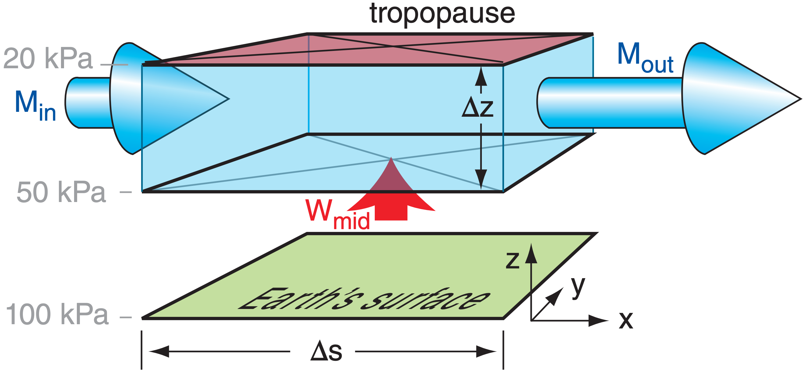
Net vertical inflow can compensate for net horizontal outflow. In the troposphere, most of this inflow happens at mid-levels (P ≈ 50 kPa) as an upward vertical velocity (W_mid). Not much vertical inflow happens across the tropopause because vertical motion in the stratosphere is suppressed by the strong static stability. In the idealized illustration of Fig. 13.29, the inflows [(M_in times the area across which the inflow occurs) plus (W_mid times its area of inflow)] equals the outflow (M_out times the outflow area).

The continuity equation describes volume conservation for this situation as

\(\ \begin{align} W_{m i d}=D \cdot \Delta z\tag{13.15}\end{align}\)

or

\(\ \begin{align} W_{m i d}=\left[\frac{\Delta U}{\Delta x}+\frac{\Delta V}{\Delta y}\right] \cdot \Delta z\tag{13.16}\end{align}\)

or

\(\ \begin{align} W_{m i d}=\frac{\Delta M}{\Delta s} \cdot \Delta z\tag{13.17}\end{align}\)

where the distance between outflow and inflow locations is ∆s, wind speed is M, the thickness of the upper air layer is ∆z, and the ascent speed at 50 kPa (mid-troposphere) is W_mid.

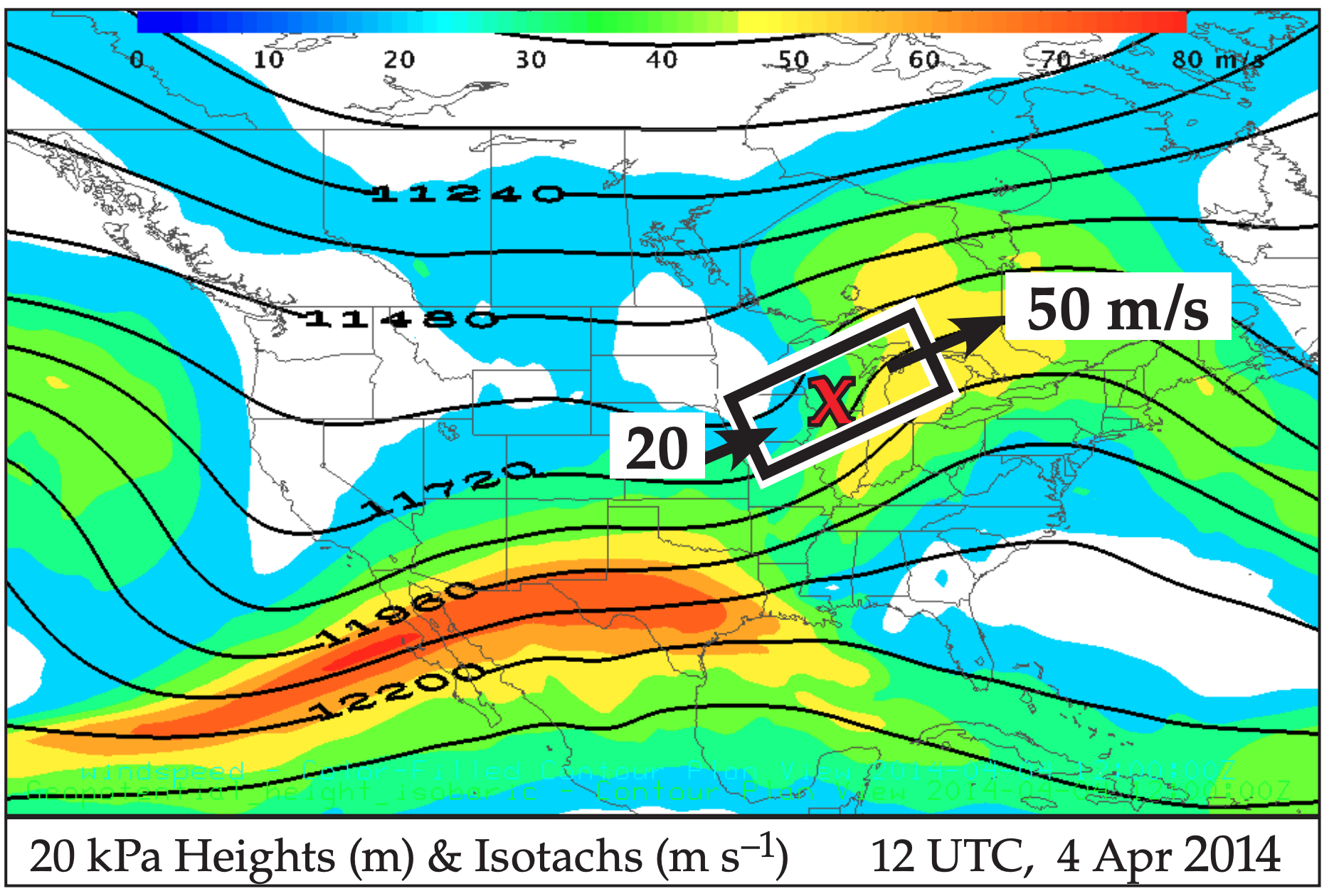
Fig. 13.30 shows this scenario for the case-study storm. Geostrophic winds are often nearly parallel to the height contours (solid black curvy lines in Fig. 13.30). Thus, for the region outlined with the black/ white box drawn parallel to the contour lines, the main inflow and outflow are at the ends of the box (arrows). The isotachs (shaded) tell us that the inflow (≈ 20 m s^–1) is slower than outflow (≈50 m s^–1).

Figure 13.30 Over the surface cyclone (X) is a region (box) with faster jetstream outflow than inflow (arrows). Isotachs are shaded.

We will focus on two processes that cause horizontal divergence of the jet stream:

• Rossby waves, a planetary-scale feature for which the jet stream is approximately geostrophic; and
• jet streaks, where jet-stream accelerations cause non-geostrophic (ageostrophic) motions.

13.5.1.1. Rossby Waves

From the Forces and Winds chapter, recall that the gradient wind is faster around ridges than troughs, for any fixed latitude and horizontal pressure gradient. Since Rossby waves consist of a train of ridges and troughs in the jet stream, you can anticipate that along the jet-stream path the winds are increasing and decreasing in speed.

Figure 13.31 Sketch showing how the slower jet-stream winds at the trough (thin lines with arrows) are enhanced by vertical velocity (W, dotted lines) to achieve the mass balance needed to support the faster winds (thick lines with arrows) at the ridge. (N. Hem.)

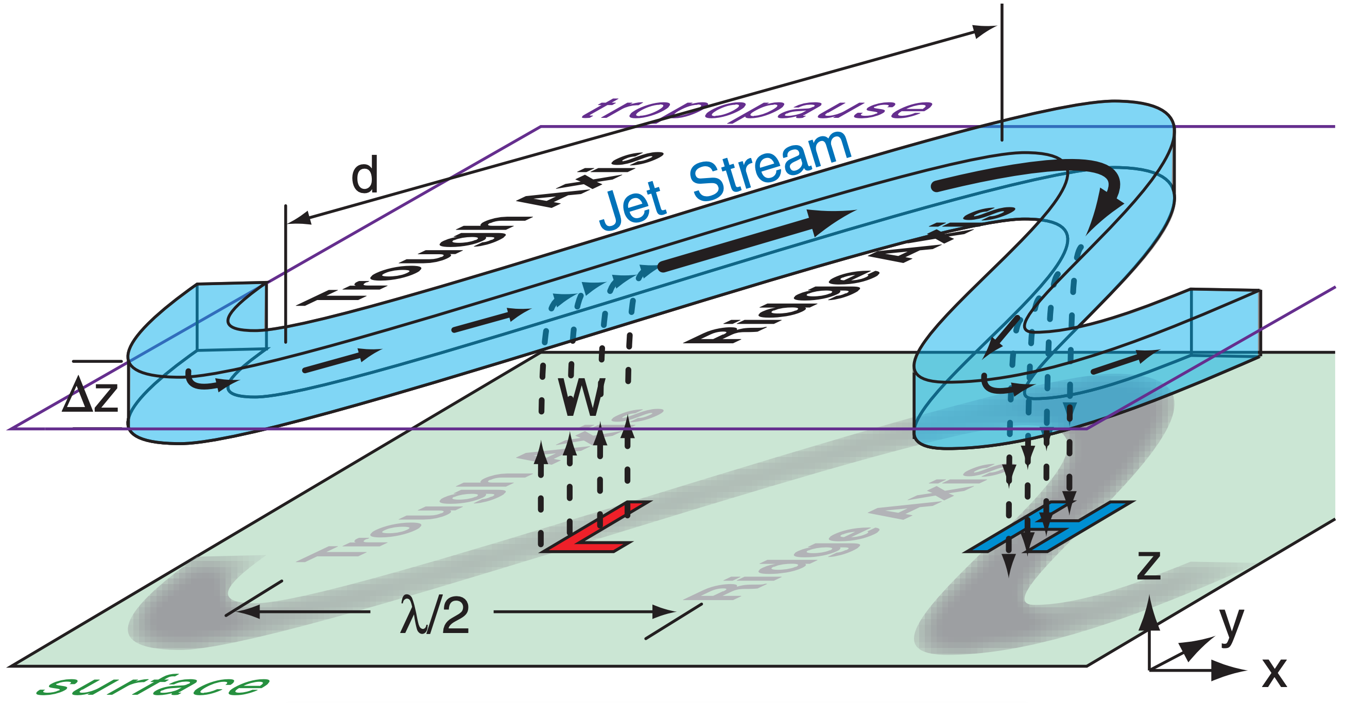
One such location is east of troughs, as sketched in Fig. 13.31. Consider a hypothetical box of air at the jet stream level between the trough and ridge. Horizontal wind speed entering the box is slow around the trough, while exiting winds are fast around the ridge. To maintain mass continuity, this horizontal divergence induces ascent into the bottom of the hypothetical box. This ascent is removing air molecules below the hypothetical box, creating a region of low surface pressure. Hence, surface lows (extratropical cyclones) form east of jet-stream troughs.

We can create a toy model of this effect. Suppose the jet stream path looks like a sine wave of wavelength λ and amplitude ∆y/2. Assume that the streamwise length of the hypothetical box equals the diagonal distance between the trough and ridge

\(\ \begin{align} \Delta s=d=\left[(\lambda / 2)^{2}+\Delta y^{2}\right]^{1 / 2}\tag{13.18}\end{align}\)

Knowing the decrease/increase relative to the geostrophic wind speed G of the actual gradient wind M around troughs/ridges (from the Forces and Winds chapter), you can estimate the jet-stream wind-speed increase as:

\(\ \begin{align} \Delta M=0.5 \cdot f_{c} \cdot R \cdot[{2-\sqrt{1-\frac{4 \cdot G}{f_{c} \cdot R}}-\sqrt{1+\frac{4 \cdot G}{f_{c} \cdot R}}}]\tag{13.19}\end{align}\)

For a simple sine wave, the radius-of-curvature R of the jet stream around the troughs and ridges is:

\(\ \begin{align} R=\frac{1}{2 \pi^{2}} \cdot \frac{\lambda^{2}}{\Delta y}\tag{13.20}\end{align}\)

Combining these equations with eq. (13.17) gives a toy-model estimate of the vertical motion:

\(\ \begin{align} W_{\text {mid}}=\frac{\frac{f_{c} \cdot \Delta z \cdot \lambda^{2}}{4 \pi^{2} \cdot \Delta y}[2-\sqrt{1-\frac{8 \pi^{2} G \cdot \Delta y}{f_{c} \cdot \lambda^{2}}}-\sqrt{1+\frac{8 \pi^{2} G \cdot \Delta y}{f_{c} \cdot \lambda^{2}}}]}{\left[(\lambda / 2)^{2}+\Delta y^{2}\right]^{1 / 2}}\tag{13.21}\end{align}\)

For our case-study cyclone, Fig. 13.30 shows a short-wave trough with jet-stream speed increasing from 20 to 50 m/s across a distance of about 1150 km. This upper-level divergence supported cyclogenesis of the surface low over Wisconsin (“X” on the map).

Sample Application

Suppose a jet stream meanders in a sine wave pattern that has a 150 km north-south amplitude, 3000 km wavelength, 3 km depth, and 35 m s^–1 mean geostrophic velocity. The latitude is such that f_c = 0.0001 s^–1 . Estimate the ascent speed under the jet.

Find the Answer

Given: ∆y = 2 · (150 km) = 300 km, λ = 3000 km, ∆z = 3 km, G = 35 m s^–1, f_c = 0.0001 s^–1.

Find: W_mid = ? m s^–1

Apply eq. (13.20):

\(R=\frac{1}{2 \pi^{2}} \cdot \frac{(3000 \mathrm{km})^{2}}{(300 \mathrm{km})}=1520 \mathrm{km}\)

Simplify eq. (13.19) by using the curvature Rossby number from the Forces and Winds chapter:

\(\frac{G}{f_{\mathcal{C}} \cdot R}=R o_{\mathcal{C}}=\frac{35 \mathrm{m} / \mathrm{s}}{\left(0.0001 \mathrm{s}^{-1}\right) \cdot\left(1.52 \times 10^{6} \mathrm{m}\right)}=0.23\)

Next, use eq. (13.19), but with Ro_c:

\(\Delta M=\frac{35 \mathrm{m} / \mathrm{s}}{2(0.23)} \cdot[2-\sqrt{1-4(0.23)}-\sqrt{1+4(0.23)}]\)

= 76.1(m/s)·[2 – 0.283 – 1.386] = 25.2 m s^–1.

Apply eq. (13.18):

d = [ (1500km)² + (300km)² ]^1/2 = 1530 km

Finally, use eq. (13.17):

\(W_{m i d}=\left(\frac{25.2 \mathrm{m} / \mathrm{s}}{1530 \mathrm{km}}\right) \cdot 3 \mathrm{km}=\underline{0.049} \mathrm{ms}^{-1}\)

Check: Physics, units, & magnitudes are reasonable.

Exposition: This ascent speed is 5 cm s^–1, which seems slow. But when applied under the large area of the jet stream trough-to-ridge region, a large amount of air mass is moved by this updraft.

13.5.1.2. Jet Streaks

The jet stream does not maintain constant speed in the jet core (center region with maximum speeds). Instead, it accelerates and decelerates as it blows around the world in response to changes in horizontal pressure gradient and direction. The fastwind regions in the jet core are called jet streaks. The response of the wind to these speed changes is not instantaneous, because the air has inertia.

Suppose the wind in a weak-pressure-gradient region had reached its equilibrium wind speed as given by the geostrophic wind. As this air coasts into a region of stronger pressure gradient (i.e., tighter packing of the isobars or height contours), it finds itself slower than the new, faster geostrophic wind speed. Namely, it is ageostrophic (not geostrophic) for a short time while it accelerates toward the faster geostrophic wind speed.

When the air parcel is too slow, its Coriolis force (which is proportional to its wind speed) is smaller than the new larger pressure gradient force. This temporary imbalance turns the air at a small angle toward lower pressure (or lower heights). This is what happens as air flows into a jet streak.

The opposite happens as air exits a jet streak and flows into a region of weaker pressure gradient. The wind is temporarily too fast because of its inertia, so the Coriolis force (larger than pressure-gradient force) turns the wind at a small angle toward higher pressure.

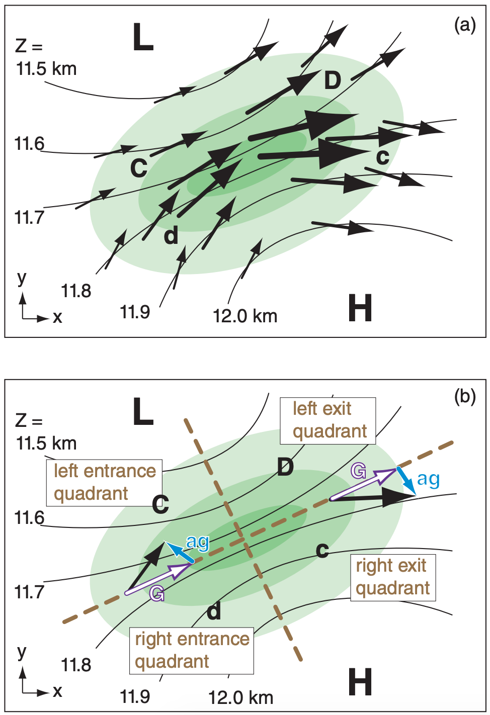
For northern hemisphere jet streams, the wind vectors point slightly left of geostrophic while accelerating, and slightly right while decelerating. Because the air in different parts of the jet streak have different wind speeds and pressure gradients, they deviate from geostrophic by different amounts (Fig. 13.32a). As a result, some of the wind vectors converge in speed and/or direction to make horizontal convergence regions. At other locations the winds cause divergence. The jet-stream divergence regions drive cyclogenesis near the Earth’s surface.

Figure 13.32 Horizontal divergence (D = strong, d = weak) and convergence (C = strong, c = weak) near a jet streak. Back arrows represent winds, green shading indicates isotachs (with the fastest winds having the darkest green), thin curved black lines are height contours of the 20 kPa isobaric surface, L & H indicate low & high height centers. Geostrophic (G) winds are parallel to the isobars, while (ag) indicates the ageostrophic wind component. Tan dashed lines parallel and perpendicular to the jet axis divide the jet streak into quadrants.

For an idealized west-to-east, steady-state jet stream with no curvature, the U-wind forecast equation (10.51a) from the Atmospheric Forces and Wind chapter reduces to:

\(\ \begin{align} 0=-U \frac{\Delta U}{\Delta x}+f_{c}\left(V-V_{g}\right)\tag{13.22}\end{align}\)

Let (U_ag, V_ag ) be the ageostrophic wind components

\(\ \begin{align} V_{a g}=V-V_{g}\tag{13.23}\end{align}\)

\(\ \begin{align} U_{a g}=U-U_{g}\tag{12.24}\end{align}\)

Plugging these into eq. (13.22) gives for a jet stream from the west:

\(\ \begin{align} V_{a g}=\frac{U}{f_{c}} \cdot \frac{\Delta U}{\Delta x}\tag{13.25}\end{align}\)

Similarly, the ageostrophic wind for south-to-north jet stream axis is

\(\ \begin{align} U_{a g}=-\frac{V}{f_{c}} \cdot \frac{\Delta V}{\Delta y}\tag{13.26}\end{align}\)

For example, consider the winds approaching the jet streak (i.e., in the entrance region) in Fig. 13.32a. The air moves into a region where U is positive and increases with x, hence V_ag is positive according to eq. (13.25). Also, V is positive and increases with y, hence, U_ag is negative. The resulting ageostrophic entrance vector is shown in blue in Fig. 13.32b. Similar analyses can be made for the jet-streak exit regions, yielding the corresponding ageostrophic wind component.

Sample Application

A west wind of 60 m s^–1 in the center of a jet streak decreases to 40 m s^–1 in the jet exit region 500 km to the east. Find the exit ageostrophic wind component.

Find the Answer

Given: ∆U = 40–60 m s^–1 = –20 m s^–1, ∆x = 500 km

Find: V_ag = ? m s^–1

Use eq. (13.25), and assume f_c = 10^–4 s^–1.

The average wind is U = (60 + 40 m s^–1)/2 = 50 m s^–1. V_ag = [(50 m s^–1) / (10^–4 s^–1)] · [( –20 m s^–1) / (5x10⁵ m)] = –20 m s^–1

Check: Physics and units are reasonable. Sign OK.

Exposition: Negative sign means V_ag is north wind.

When considering a jet streak, imagine it divided into the four quadrants sketched in Fig. 13.32 (also Fig. 13.35). The combination of speed and direction changes cause strong divergence in the left exit quadrant, and weaker divergence in the right entrance quadrant. These are the regions where cyclogenesis is favored under the jet. Cyclolysis is favored under the convergence regions of the right exit and left entrance regions.

This ageostrophic behavior can also be seen in the maps for a different case-study (Fig. 13.33). This figure overlays wind vectors, isotachs, and geopotential height contours near the top of the troposphere (at 20 kPa). The broad area of shading shows the jet stream. Embedded within it are two relative speed maxima (one over Texas, and the other over New England) that we identify as jet streaks. Recall that if winds are geostrophic (or gradient), then they should flow parallel to the height contours.

Figure 13.33 (Not the 2014 case study.) Superposition of the 20 kPa charts for geopotential heights (medium-thickness black curved lines), isotachs in m s^–1 (shading), and winds (vectors). The scale for winds and the values for the height contours are identical to those in Figs. 13.17. Regions of relatively darker shading indicate the jet streaks. White/black square outlines the exit region from a small jet streak over Texas, and white/black oval outlines the entrance region for a larger jet streak over the northeastern USA.

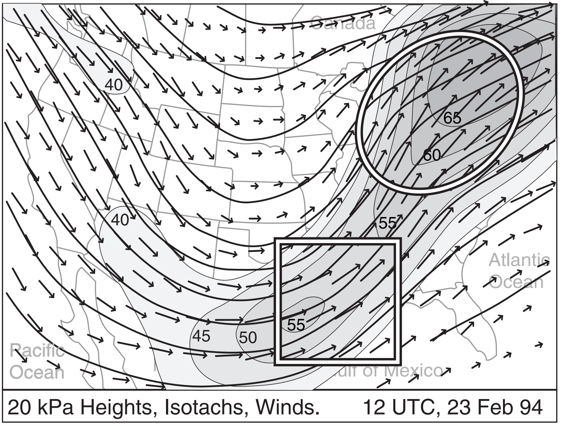
In Fig. 13.33 the square highlights the exit region of the Texas jet streak, showing wind vectors that cross the height contours toward the right. Namely, inertia has caused these winds to be faster than geostrophic (supergeostrophic), therefore Coriolis force is stronger than pressure-gradient force, causing the winds to be to the right of geostrophic. The oval highlights the entrance region of the second jet, where winds cross the height contours to the left. Inertia results in slower-than-geostrophic winds (subgeostrophic), causing the Coriolis force to be too weak to counteract pressure-gradient force.

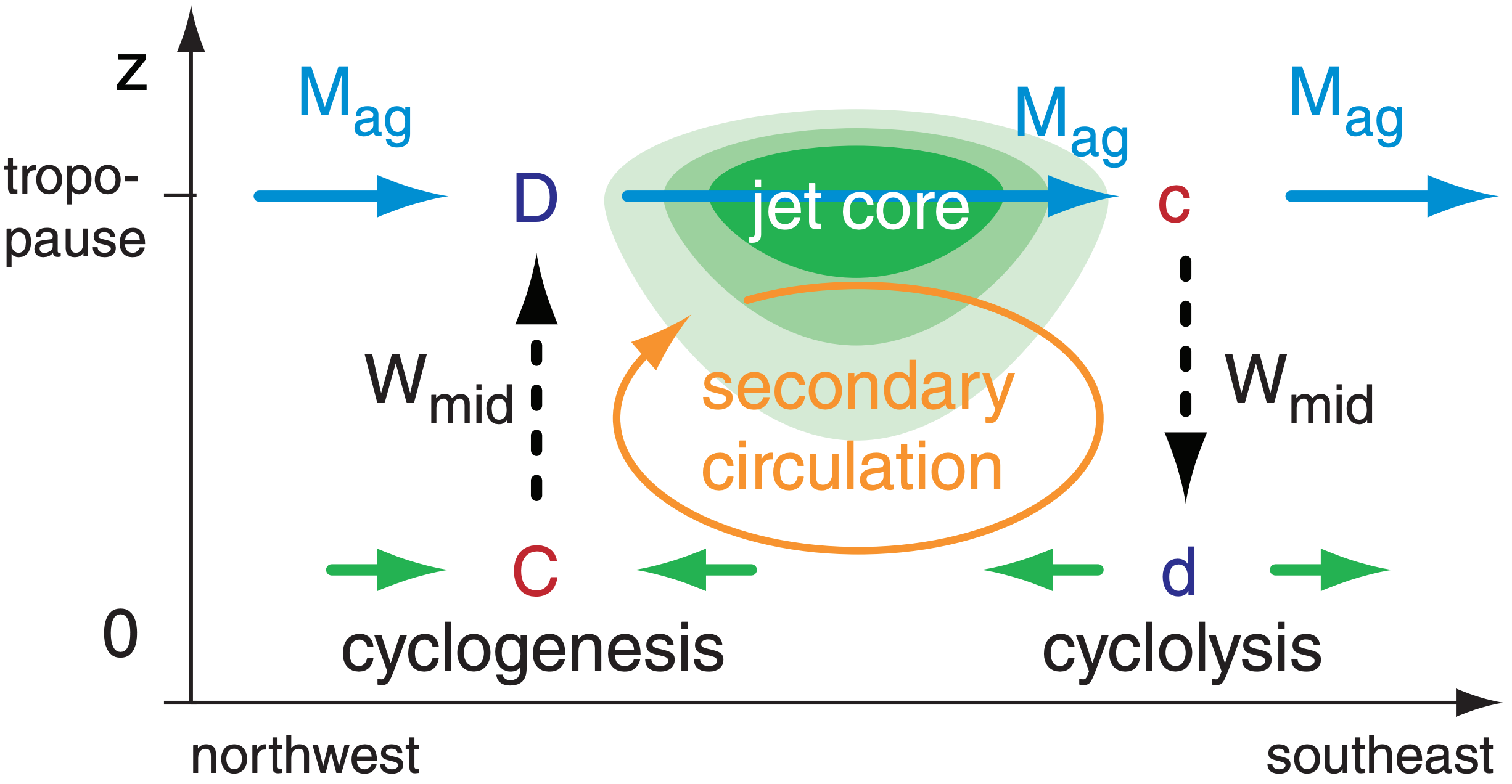
Consider a vertical slice through the atmosphere, perpendicular to the geostrophic wind at the jet exit region (Fig. 13.32). The resulting combination of ageostrophic winds (M_ag) induce mid-tropospheric ascent (W_mid) and descent that favors cyclogenesis and cyclolysis, respectively (Fig. 13.34). The weak, vertical, cross-jet flow (orange in Fig. 13.34) is a secondary circulation.

Figure 13.34 Vertical slice through the atmosphere at the jet-streak exit region, perpendicular to the average jet direction. Viewed from the west southwest, the green shading indicates isotachs of the jet core into the page. Divergence (D) in the left exit region creates ascent (W, dotted lines) to conserve air mass, which in turn removes air from near the surface. This causes the surface pressure to drop, favoring cyclogenesis. The opposite happens under the right exit region, where cyclolysis is favored.

INFO • Ageostrophic right-hand rule

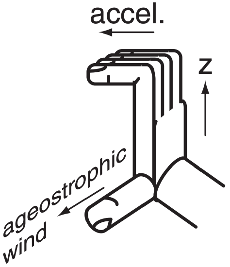
If the geostrophic winds are accelerating, use your right hand to curl your fingers from vertical toward the direction of acceleration (the acceleration vector). Your thumb points in the direction of the ageostrophic wind.

This right-hand rule also works for deceleration, for which case the direction of acceleration is opposite to the wind direction.

Figure g.

The secondary circulation in the jet exit region is opposite to the Hadley cell rotation direction in that hemisphere; hence, it is called an indirect circulation. In the jet entrance region is a direct secondary circulation.

Figure 13.35 (Not the 2014 case study.) Entrance and exit regions of jet streaks (highlighted with ovals). X marks the surface low center.

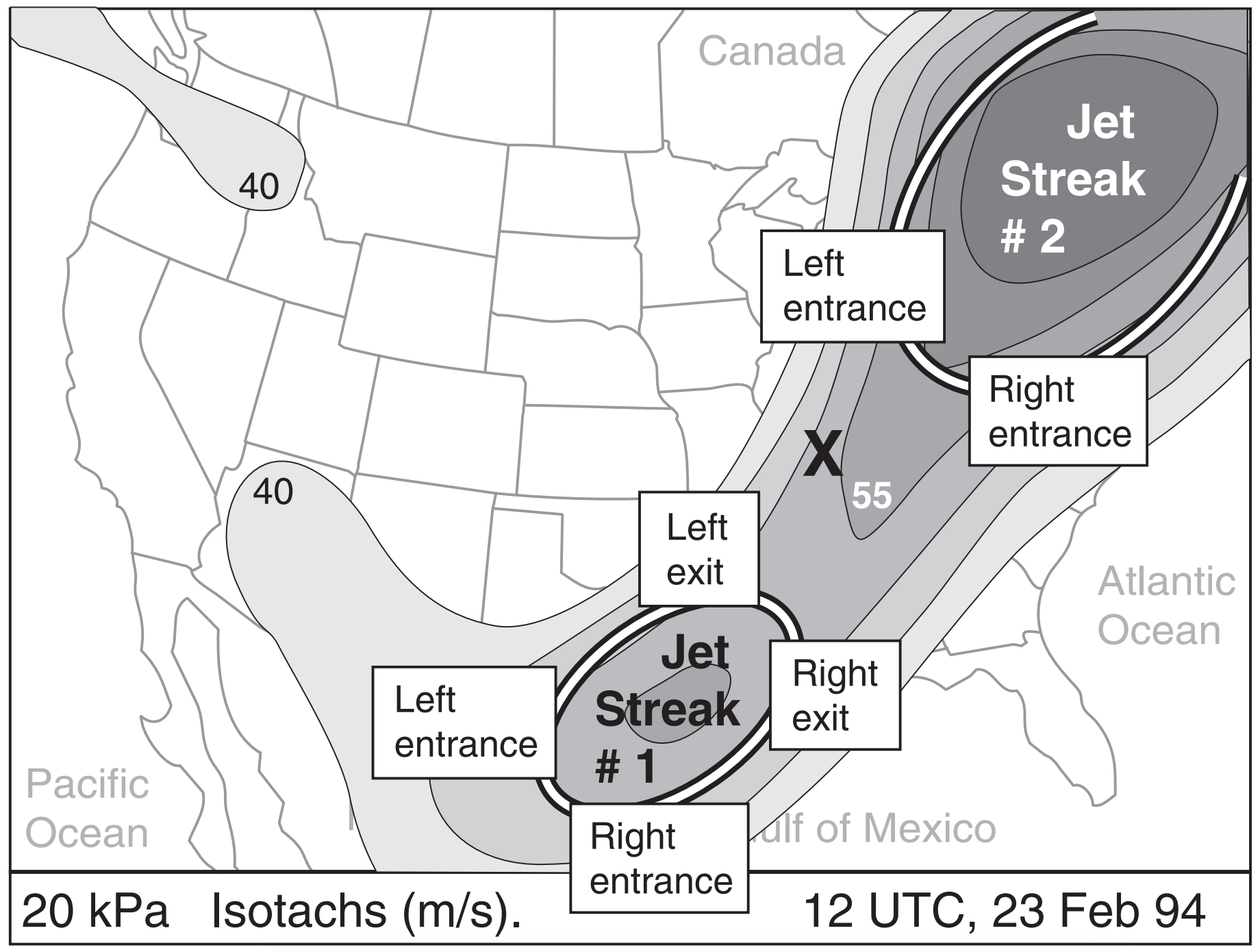
Looking again at the 23 Feb 1994 weather maps, Fig. 13.35 shows the entrance and exit regions of the two dominant jet streaks in this image (for now, ignore the smaller jet streak over the Pacific Northwest). Thus, you can expect divergence aloft at the left exit and right entrance regions. These are locations that would favor cyclogenesis near the ground. Indeed, a new cyclone formed over the Carolinas (under the right entrance region of jet streak # 2). Convergence aloft, favoring cyclolysis (cyclone death), is at the left entrance and right exit regions.

You can estimate mid-tropospheric ascent (W_mid) under the right entrance and left exit regions as follows. Define ∆s = ∆y as the north-south half-width of a predominantly west-to-east jet streak. As you move distance ∆y to the side of the jet, suppose that V_ag gradually reduces to 0. Combining eqs. (13.25) and (13.16) with V_ag in place of M, the mid-tropospheric ascent driven by the jet streak is

\(\ \begin{align} W_{m i d}=\left|\frac{U \cdot \Delta U}{f_{c} \cdot \Delta x}\right| \cdot \frac{\Delta z}{\Delta y}\tag{13.27}\end{align}\)

Sample Application

A 40 m s^–1 in a jet core reduces to 20 m s^–1 at 1,200 km downstream, at the exit region. The jet cross section is 4 km thick and 800 km wide. Find the mid-tropospheric ascent. f_c = 10^–4 s^–1.

Find the Answer

Given: ∆U = 20 – 40 = –20 m s^–1, U = 40 m s^–1, f_c = 10^–4 s^–1, ∆z = 4km, ∆y = 800 km, ∆x = 1.2x106 m.

Find: W_mid = ? m s^–1

Use eq. (13.27):

\(W_{\text {mid}}=\left|\frac{(40 \mathrm{m} / \mathrm{s}) \cdot(-20 \mathrm{m} / \mathrm{s})}{\left(10^{-4} \mathrm{s}^{-1}\right) \cdot\left(1.2 \times 10^{6} \mathrm{m}\right)}\right| \cdot \frac{(4 \mathrm{km})}{(800 \mathrm{km})}=0.033 \mathrm{m} \mathrm{s}^{-1}\)

Check: Physics and units are reasonable.

Exposition: This small ascent speed, when active over a day or so, can be important for cyclogenesis.

INFO • Sutcliffe Development Theorem

To help forecast cyclogenesis, Sutcliffe devised

\(D_{t o p}-D_{b o t t o m}=-\frac{1}{f_{c}}\left[U_{T H} \frac{\Delta \zeta_{g c}}{\Delta x}+V_{T H} \frac{\Delta \zeta_{g c}}{\Delta y}\right]\)

where divergence is D = ∆U/∆x + ∆V/∆y, column geostrophic vorticity is ζ_gc = ζ_{g top} + ζ_{g bottom} + f_c , and (U_TH, V_TH) are the thermal-wind components.

This says that if the vorticity in an air column is positively advected by the thermal wind, then this must be associated with greater air divergence at the column top than bottom. When combined with eq. (13.15), this conclusion for upward motion is nearly identical to that from the Trenberth omega eq. (13.29).

13.5.2. Omega Equation

The omega equation is the name of a diagnostic equation used to find vertical motion in pressure units (omega; ω). We will use a form of this equation developed by K. Trenberth, based on quasi-geostrophic dynamics and thermodynamics.

The full omega equation is one of the nastierlooking equations in meteorology (see the HIGHER MATH box). To simplify it, focus on one part of the full equation, apply it to the bottom half of the troposphere (the layer between 100 to 50 kPa isobaric surfaces), and convert the result from ω to W.

The resulting approximate omega equation is:

\(\ \begin{align} W_{m i d} \cong \frac{-2 \cdot \Delta z}{f_{c}}\left[U_{T H} \frac{\overline{\Delta \zeta_{g}}}{\Delta x}+V_{T H} \frac{\overline{\Delta \zeta_{g}}}{\Delta y}+V_{T H} \frac{\beta}{2}\right]\tag{13.28}\end{align}\)

where W_mid is the vertical velocity in the mid-troposphere (at P = 50 kPa), ∆z is the 100 to 50 kPa thickness, U_TH and V_TH are the thermal-wind components for the 100 to 50 kPa layer, f_c is Coriolis parameter, β is the change of Coriolis parameter with y (see eq. 13.2), ζ_g is the geostrophic vorticity, and the overbar represents an average over the whole depth of the layer. An equivalent form is:

\(\ \begin{align} W_{m i d} \cong \frac{-2 \cdot \Delta z}{f_{c}}\left[M_{T H} \frac{\overline{\Delta\left(\zeta_{g}+\left(f_{c} / 2\right)\right.})}{\Delta s}\right]\tag{13.29}\end{align}\)

where s is distance along the thermal wind direction, and M_TH is the thermal-wind speed.

Sample Application

The 100 to 50 kPa thickness is 5 km and f_c = 10^–4 s^–1. A west to east thermal wind of 20 m s^–1 blows through a region where avg. cyclonic vorticity decreases by 10^–4 s^–1 toward the east across a distance of 500 km. Use the omega eq. to find mid-tropospheric upward speed.

Find the Answer

Given: U_TH = 20 m s^–1, V_TH = 0, ∆z = 5 km, ∆ζ = –10^–4 s^–1 , ∆x = 500 km, f_c = 10^–4 s^–1.

Find: W_mid = ? m s^–1

Use eq. (13.28):

\(W_{m i d} \cong \frac{-2 \cdot(5000 m)}{\left(10^{-4} s^{-1}\right)}\left[(20 m / s) \frac{\left(-10^{-4} s^{-1}\right)}{\left(5 \times 10^{5} m\right)}+0+0\right]=\underline{0.4 m s^{-1}}\)

Check: Units OK. Physics OK.

Exposition: At this speed, an air parcel would take 7.6 h to travel from the ground to the tropopause.

Regardless of the form, the terms in square brackets represent the advection of vorticity by the thermal wind, where vorticity consists of the geostrophic relative vorticity plus a part of the vorticity due to the Earth’s rotation. The geostrophic vorticity at the 85 kPa or the 70 kPa isobaric surface is often used to approximate the average geostrophic vorticity over the whole 100 to 50 kPa layer.

A physical interpretation of the omega equation is that greater upward velocity occurs where there is greater advection of cyclonic (positive) geostrophic vorticity by the thermal wind. Greater upward velocity favors clouds and heavier precipitation. Also, by moving air upward from the surface, it reduces the pressure under it, causing the surface low to move toward that location and deepen.

Figure 13.36 (a) Weather at three different pressure heights: (1) 50 kPa heights (solid blue lines) and trough axis (thick dashed line); (2) surface low pressure center (L) and fronts; (3) 70 kPa vorticity (shaded). (b) Trough axis, surface low and fronts, and vorticity shading are identical to Fig. (a). Added are: 100 to 50 kPa thickness (dotted green lines), thermal wind vectors (arrows), and region of maximum positive vorticity advection by the thermal wind (rectangular box). It is within this box that the omega equation gives the greatest updraft speed, which supports cyclogenesis.

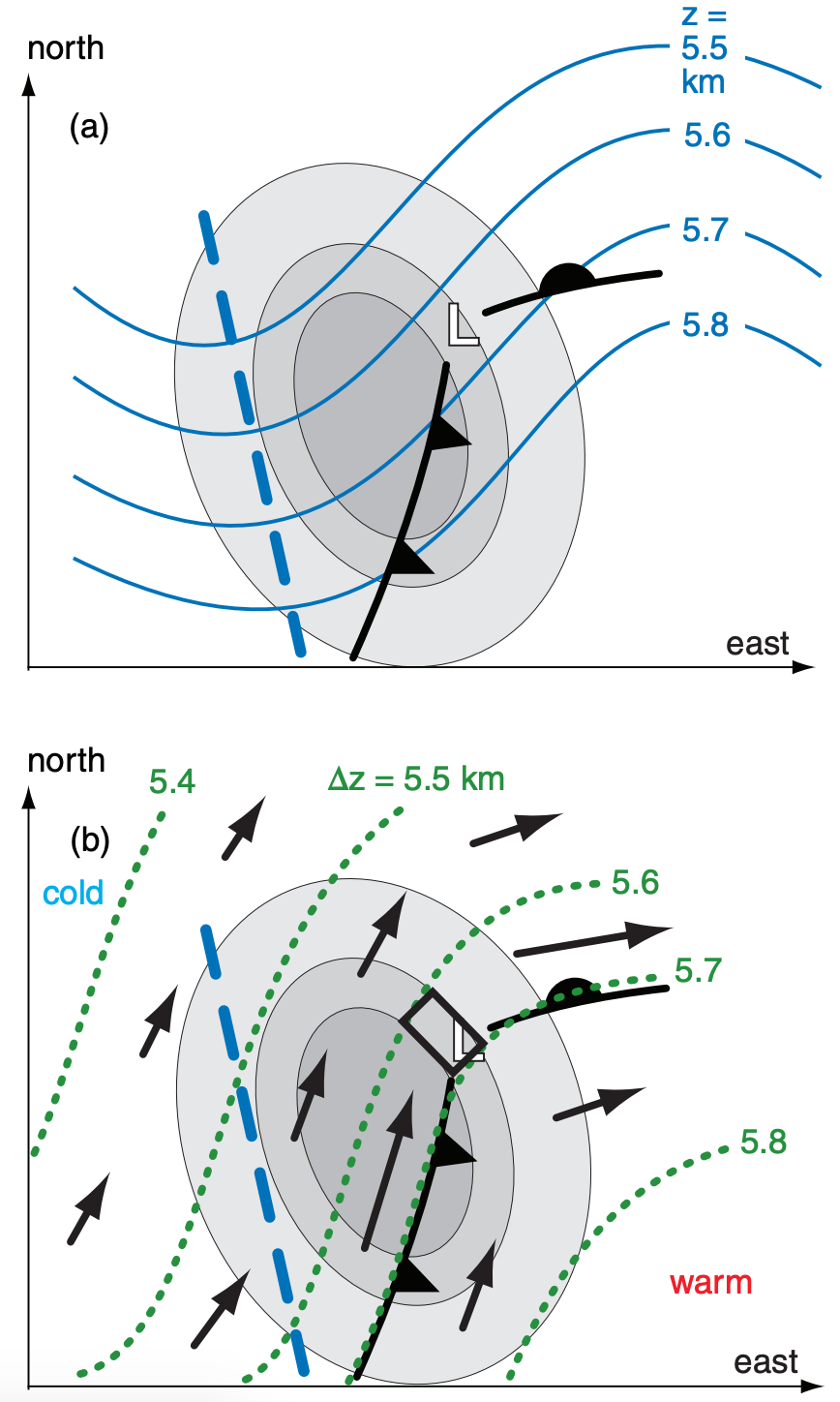
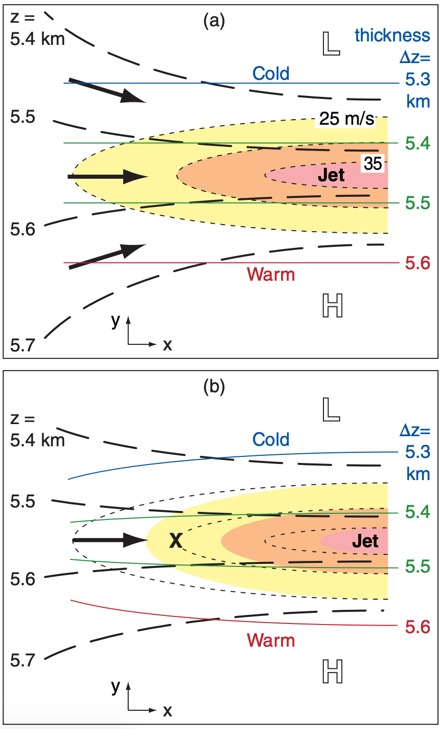
Weather maps can be used to determine the location and magnitude of the maximum upward motion. The idealized map of Fig. 13.36a shows the height (z) contours of the 50 kPa isobaric surface, along with the trough axis. Also shown is the location of the surface low and fronts.

At the surface, the greatest vorticity is often near the low center. At 50 kPa, it is often near the trough axis. At 70 kPa, the vorticity maximum (vort max) is usually between those two locations. In Fig. 13.36a, the darker shading corresponds to regions of greater cyclonic vorticity at 70 kPa.

Fig. 13.36b shows the thickness (∆z) of the layer of air between the 100 and 50 kPa isobaric surfaces. Thickness lines are often nearly parallel to surface fronts, with the tightest packing on the cold side of the fronts. Recall that thermal wind is parallel to the thickness lines, with cold air to the left, and with the greatest velocity where the thickness lines are most tightly packed. Thermal wind direction is represented by the arrows in Fig. 13.36b, with longer arrows denoting stronger speed.

Advection is greatest where the area between crossing isopleths is smallest (the INFO Box on the next page explains why). This rule also works for advection by the thermal wind. The dotted lines represent the isopleths that drive the thermal wind. In Fig. 13.36 the thin black lines around the shaded areas are isopleths of vorticity. The solenoid at the smallest area between these crossing isopleths indicates the greatest vorticity advection by the thermal wind, and is outlined by a rectangular box. For this particular example, the greatest updraft would be expected within this box.

HIGHER MATH • The Omega Eq.

Full Omega Equation

The omega equation describes vertical motion in pressure coordinates. One form of the quasi-geostrophic omega equation is:

\(\begin{aligned}\left\{\nabla_{p}^{2}+\frac{f_{o}^{2}}{\sigma} \frac{\partial^{2}}{\partial p^{2}}\right\} \omega &=\frac{-f_{0}}{\sigma} \cdot \frac{\partial}{\partial p}\left[-\vec{V}_{g} \cdot \vec{\nabla}_{p}\left(\zeta_{g}+f_{c}\right)\right] - \frac{\Re}{\sigma \cdot p} \cdot \nabla_{p}^{2}\left[-\vec{V}_{g} \cdot \vec{\nabla}_{p} T\right] \end{aligned}\)

where f_o is a reference Coriolis parameter f_c at the center of a beta plane, σ is a measure of static stability, Vg is a vector geostrophic wind, ℜ is the ideal gas law constant, p is pressure, T is temperature, ζ_g is geostrophic vorticity, and • means vector dot product.

\(\vec{\nabla}_{p}()=\partial() /\left.\partial x\right|_{p}+\partial() /\left.\partial y\right|_{p}\) is the del operator, which gives quasi-horizontal derivatives along an isobaric surface. Another operator is the Laplacian:

\(\nabla^{2}_{p}()=\partial^{2}() /\left.\partial x^{2}\right|_{p}+\partial^{2}() /\left.\partial y^{2}\right|_{p}\)

Although the omega equation looks particularly complicated and is often shown to frighten unsuspecting people, it turns out to be virtually useless. The result of this equation is a small difference between very large terms on the RHS that often nearly cancel each other, and which can have large error.

Trenberth Omega Equation

Trenberth developed a more useful form that avoids the small difference between large terms:

\(\left\{\nabla_{p}^{2}+\frac{f_{o}^{2}}{\sigma} \frac{\partial^{2}}{\partial p^{2}}\right\} \omega=\frac{2 f_{0}}{\sigma} \cdot\left[\frac{\partial \vec{V}_{g}}{\partial p} \cdot \vec{\nabla}_{p}\left(\zeta_{g}+\left(f_{c} / 2\right)\right)\right]\)

For the omega subsection of this chapter, we focus on the vertical (pressure) derivative on the LHS, and ignore the Laplacian. This leaves:

\(\frac{f_{o}^{2}}{\sigma} \frac{\partial^{2} \omega}{\partial p^{2}}=\frac{2 f_{0}}{\sigma} \cdot\left[\frac{\partial \vec{V}_{g}}{\partial p} \cdot \vec{\nabla}_{p}\left(\zeta_{g}+\left(f_{c} / 2\right)\right)\right]\)

Upon integrating over pressure from p = 100 to 50 kPa:

\(\frac{\partial \omega}{\partial p}=\frac{-2}{f_{o}} \cdot\left[\vec{V}_{T H} \bullet \overline{ \vec{\nabla}_{p}\left(\zeta_{g}+\left(f_{c} / 2\right)\right)}\right]\)

where the definition of thermal wind V_TH is used, along with the mean value theorem for the last term.

The hydrostatic eq. is used to convert the LHS: ∂ ∂ ω/ / p W = ∂ ∂z . The whole eq. is then integrated over height, with W = W_mid at z = ∆z (= 100 - 50 kPa thickness) and W = 0 at z = 0.

This gives

\(W_{m i d}=
\frac{-2 \cdot \Delta z}{f_{c}}\left[U_{T H} \frac{\overline{\Delta\left (\zeta_{g}+\left(f_{c} / 2\right)\right)}}{\Delta x}+V_{T H} \frac{\overline{ \Delta\left(\zeta_{g}+\left(f_{c} / 2\right)\right)}}{\Delta y}\right]\)

But f_c varies with y, not x. The result is eq. (13.28).

INFO • Max Advection on Wx Maps

One trick to locating the region of maximum advection is to find the region of smallest area between crossing isopleths on a weather (wx) map, where one set of isopleths must define a wind.

For example, consider temperature advection by the geostrophic wind. Temperature advection will occur only if the winds blow across the isotherms at some nonzero angle. Stronger temperature gradient with stronger wind component perpendicular to that gradient gives stronger temperature advection.

But stronger geostrophic winds are found where the isobars are closer together. Stronger temperature gradients are found where the isotherms are closer together. In order for the winds to cross the isotherms, the isobars must cross the isotherms. Thus, the greatest temperature advection is where the tightest isobar packing crosses the tightest isotherm packing. At such locations, the area bounded between neighboring isotherms and isobars is smallest.

This is illustrated in the surface weather map below, where the smallest area is shaded to mark the maximum temperature advection. There is a jet of strong geostrophic winds (tight isobar spacing) running from northwest to southeast. There is also a front with strong temperature gradient (tight isotherm spacing) from northeast to southwest. However, the place where the jet and temperature gradient together are strongest is the shaded area.

Each of the odd-shaped tiles (solenoids) between crossing isobars and isotherms represents the same amount of temperature advection. But larger tiles imply that temperature advection is spread over larger areas. Thus, greatest temperature flux (temperature advection per unit area) is at the smallest tiles.

This approach works for other variables too. If isopleths of vorticity and height contours are plotted on an upper-air chart, then the smallest area between crossing isopleths indicates the region of maximum vorticity advection by the geostrophic wind. For vorticity advection by the thermal wind, plot isopleths of vorticity vs. thickness contours.

Fig. h. Solid lines are isobars. Grey dashed lines are isotherms. Greatest temperature advection is at the green tile.

Be careful when you identify the smallest area. In Fig. 13.36b, another area equally as small exists further south-south-west from the low center. However, the cyclonic vorticity is being advected away from this region rather than toward it. Hence, this is a region of negative vorticity advection by the thermal wind, which would imply downward vertical velocity and cyclolysis or anticyclogenesis.

Figure 13.37 (At right. Not the 2014 case study.) Superposition of the vorticity chart (grey lines and shading) at 85 kPa with the chart for thickness (thick black lines) between the 100 and 50 kPa isobaric surfaces, for a 1994 event. The thermal wind (arrows) blows parallel to the thickness lines with cold air to its left. The white box highlights a region of positive vorticity advection (PVA) by the thermal wind, where updrafts, cyclogenesis, and bad weather would be expected.

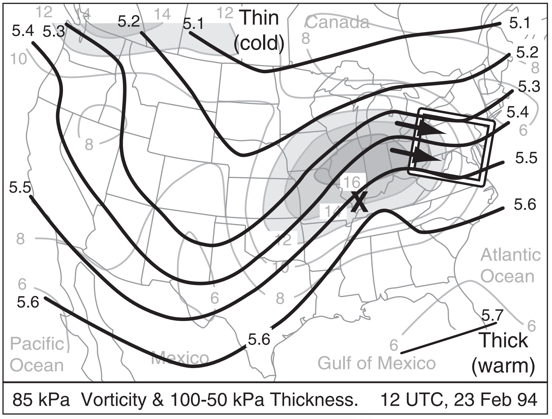
To apply these concepts to the 1994 event, Fig. 13.37 superimposes the 85 kPa vorticity chart with the 100 - 50 kPa thickness chart. The white box highlights a region of small solenoids, with the thermal wind blowing from high towards low vorticity. Hence, the white box outlines an area of positive vorticity advection (PVA) by the thermal wind, so you can anticipate substantial updrafts in that region. Such updrafts would create bad weather (clouds and precipitation), and would encourage cyclogenesis in the region outlined by the white box.

Near the surface low center (marked by the X in Fig. 13.37) is weak negative vorticity advection. This implies downdrafts, which contribute to cyclolysis. This agrees with the actual cyclone evolution, which began weakening at this time, while a new cyclone formed near the Carolinas and moved northward along the USA East Coast.

The Trenberth omega equation is heavily used in weather forecasting to help diagnose synopticscale regions of updraft and the associated cyclogenesis, cloudiness and precipitation. However, in the derivation of the omega equation (which we did not cover in this book), we neglected components that describe the role of ageostrophic motions in helping to maintain geostrophic balance. The INFO box on the Geostrophic Paradox describes the difficulties of maintaining geostrophic balance in some situations — motivation for Hoskin’s Q-vector approach described next.

INFO • The Geostrophic Paradox

Consider the entrance region of a jet streak. Suppose that the thickness contours are initially zonal, with cold air to the north and warm to the south (Fig. i(a)). As entrance winds (black arrows in Fig. i(a) converge, warm and cold air are advected closer to each other. This causes the thickness contours to move closer together (Fig. i(b), in turn suggesting tighter packing of the height contours and faster geostrophic winds at location “X” via the thermal wind equation. But the geostrophic wind in Fig. i(a) is advecting slower wind speeds to location “X”.

Paradox: advection of the geostrophic wind by the geostrophic wind seems to undo geostrophic balance at “X”.

Fig. i. Entrance region of jet streak on a 50 kPa isobaric surface. z is height (black dashed lines), ∆z is thickness (thin colored lines), shaded areas are wind speeds, with initial isotachs as dotted black lines. L & H are low and high heights. (a) Initially. (b) Later.

13.5.3. Q-Vectors

Q-vectors allow an alternative method for diagnosing vertical velocity that does not neglect as many terms.

Figure 13.38 (a) Components of a Q-vector. (b) How to recognize patterns of vector convergence (C) and divergence (D) on weather maps.

13.5.3.1. Defining Q-vectors

Define a horizontal Q-vector (units m²·s^–1·kg^–1) with x and y components as follows:

\(\ \begin{align} Q_{x}=-\frac{\Re}{P}\left[\left(\frac{\Delta U_{g}}{\Delta x} \cdot \frac{\Delta T}{\Delta x}\right)+\left(\frac{\Delta V_{g}}{\Delta x} \cdot \frac{\Delta T}{\Delta y}\right)\right]\tag{13.30}\end{align}\)

\(\ \begin{align} Q_{y}=-\frac{\Re}{P}\left[\left(\frac{\Delta U_{g}}{\Delta y} \cdot \frac{\Delta T}{\Delta x}\right)+\left(\frac{\Delta V_{g}}{\Delta y} \cdot \frac{\Delta T}{\Delta y}\right)\right]\tag{13.31}\end{align}\)

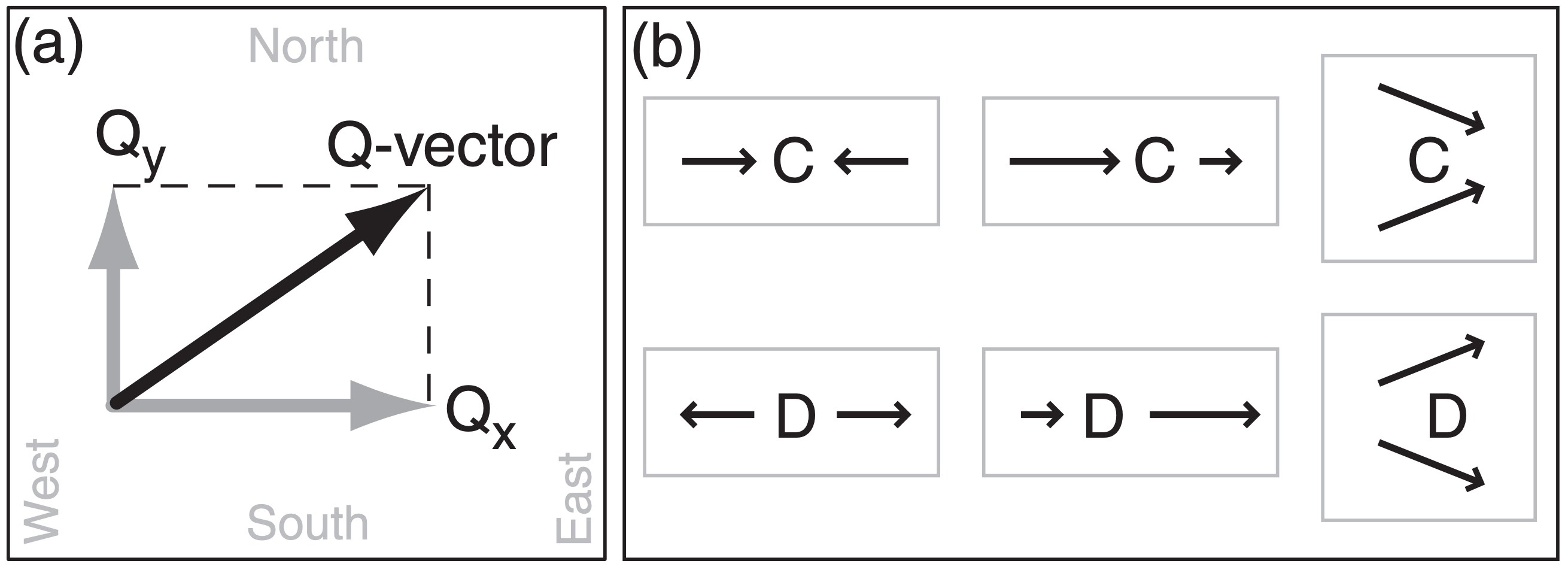
where ℜ = 0.287 kPa·K^–1·m³·kg^–1 is the gas constant, P is pressure, (U_g, V_g) are the horizontal components of geostrophic wind, T is temperature, and (x, y) are eastward and northward horizontal distances. On a weather map, the Q_x and Q_y components at any location are used to draw the Q-vector at that location, as sketched in Fig. 13.38a. Q-vector magnitude is

\(\ \begin{align} |Q|=\left(Q_{x}^{2}+Q_{y}^{2}\right)^{1 / 2}\tag{13.32}\end{align}\)

Sample Application

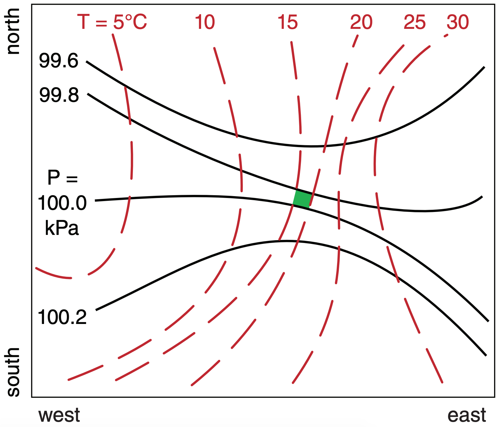
Given the weather map at right showing the temperature and geostrophic wind fields over the NE USA. Find the Q-vector at the “X” in S.E. Pennsylvania. Side of each grid square is 100 km, and corresponds to G = 5 m s^–1 for the wind vectors.

Figure j

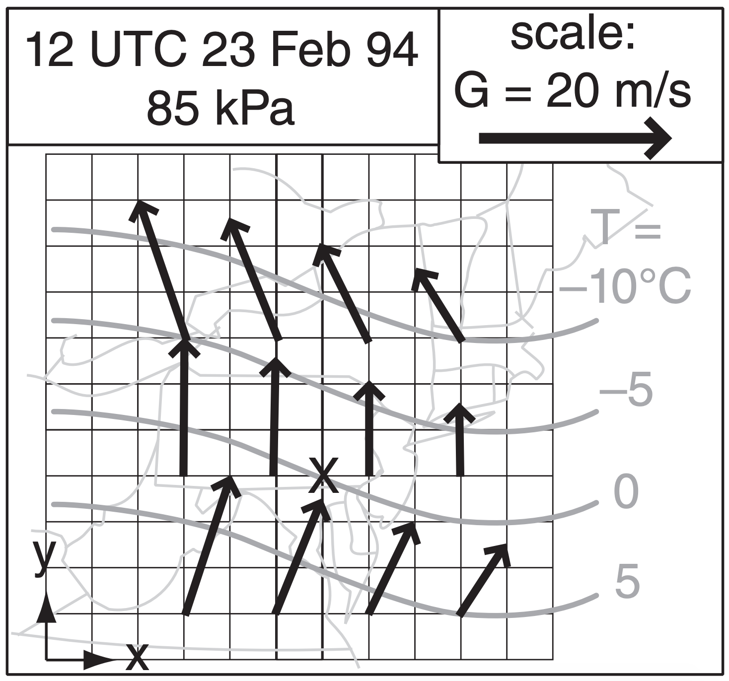
Find the Answer

Given: P = 85 kPa, G (m s^–1) & T (°C) fields on map.

Find: Q_x & Q_y = ? m² ·s^–1 ·kg^–1

First, estimate U_g, V_g, and T gradients from the map.

∆T/∆x = –5°C/600km, ∆T/∆y = –5°C/200km, ∆U_g/∆x = 0, ∆V_g/∆x = (–2.5m s^–1)/200km ∆Ug/∆y = (–5m s^–1)/300km, ∆Vg/∆y = 0, ℜ/P = 0.287/85 = 0.003376 m³·kg^–1·K^–1

Use eq. (13.30): Qx = – (0.003376 m³·kg^–1·K^–1)· [( (0)·(–8.3) + (–12.5)·(–25)]·10–12 K·m^–1·s^–1

Qx = –1.06x10^–12 m² ·s^–1 ·kg^–1

Use eq. (13.31): Qy = – (0.003376 m³·kg^–1·K^–1)· [( (–16.7)·(–8.3) + (0)·(–25)]·10^–12 K·m^–1·s^–1

Qy = –0.47x10^–12 m² ·s^–1 ·kg^–1

Use eq. (13.32) to find Q-vector magnitude:

|Q| = [(–1.06)² + (–0.47)²] ^1/2 · 10^–12 K·m^–1·s^–1

|Q| = 1.16x10^–12 m² ·s^–1 ·kg^–1

Check: Physics, units are good. Similar to Fig. 13.40.

Exposition: The corresponding Q-vector is shown at right; namely, it is pointing from the NNE because both Qx and Qy are negative. There was obviously a lot of computations needed to get this one Q-vector.

Luckily, computers can quickly compute Q-vectors for many points in a grid, as shown in Fig. 13.40. Normally, you don’t need to worry about the units of the Q-vector. Instead, just focus on Q-vector convergence zones such as computers can plot (Fig. 13.41), because these zones are where the bad weather is.

13.5.3.2. Estimating Q-vectors

Eqs. (13.30 - 13.32) seem non-intuitive in their existing Cartesian form. Instead, there is an easy way to estimate Q-vector direction and magnitude using weather maps. First, look at direction.

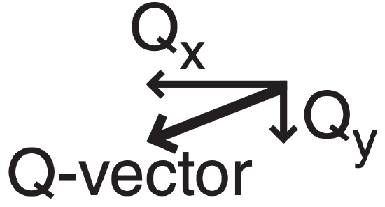
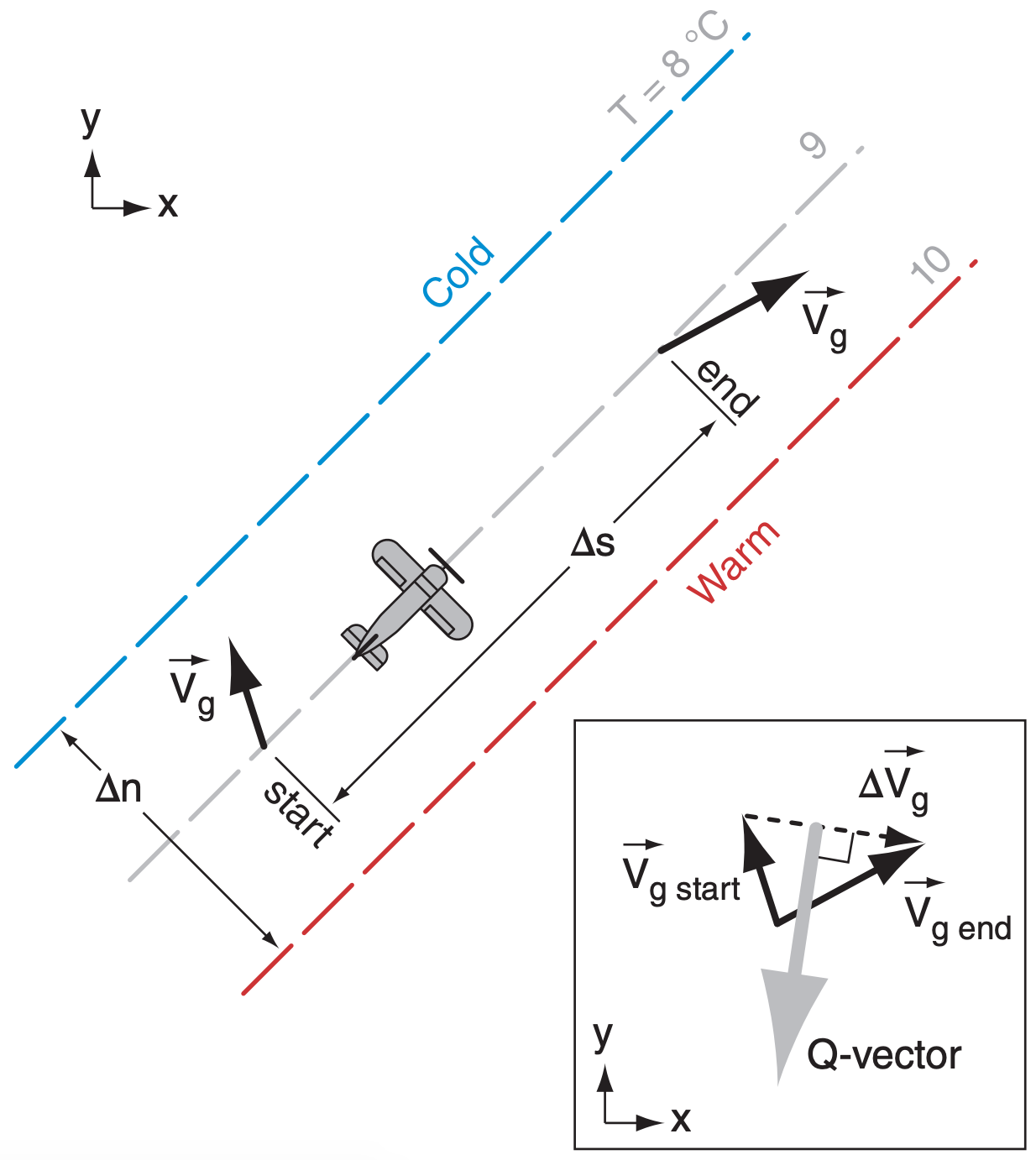
Suppose you fly along an isotherm (Fig. 13.39) in the direction of the thermal wind (in the direction that keeps cold air to your left). Draw an arrow describing the geostrophic wind vector that you observe at the start of your flight, and draw a second arrow showing the geostrophic wind vector at the end of your flight. Next, draw the vector difference, which points from the head of the initial vector to the head of the final vector. The Q-vector direction points 90° to the right (clockwise) from the geostrophic difference vector.

The magnitude is

\(\ \begin{align} |Q|=\frac{\mathfrak{R}}{P}\left|\frac{\Delta T}{\Delta n} \cdot \frac{\Delta \vec{V}_{g}}{\Delta s}\right|\tag{13.33}\end{align}\)

where ∆n is perpendicular distance between neighboring isotherms, and where the temperature difference between those isotherms is ∆T. Stronger baroclinic zones (namely, more tightly packed isotherms) have larger temperature gradient ∆T/∆n. Also, ∆s is distance of your flight along one isotherm, and ∆V_g is the magnitude of the geostrophic difference vector from the previous paragraph. Thus, greater changes of geostrophic wind in stronger baroclinic zones have larger Q-vectors. Furthermore, Q-vector magnitude increases with the decreasing pressure P found at increasing altitude.

Figure 13.39 Illustration of natural coordinates for Q-vectors. Dashed grey lines are isotherms. Aircraft flies along the isotherms with cold air to its left. Black arrows are geostrophic wind vectors. Grey arrow indicates Q-vector direction (but not magnitude).

13.5.3.3. Using Q-vectors / Forecasting Tips

Figure 13.40 (Not the 2014 case study.) Weather map of Q-vectors. (o means small magnitude.)

Figure 13.41 (Not the 2014 case study.) Convergence of Q-vectors (shaded). Divergence (dashed lines). See the Info box in section 13.1.3 for identification of geographic features.

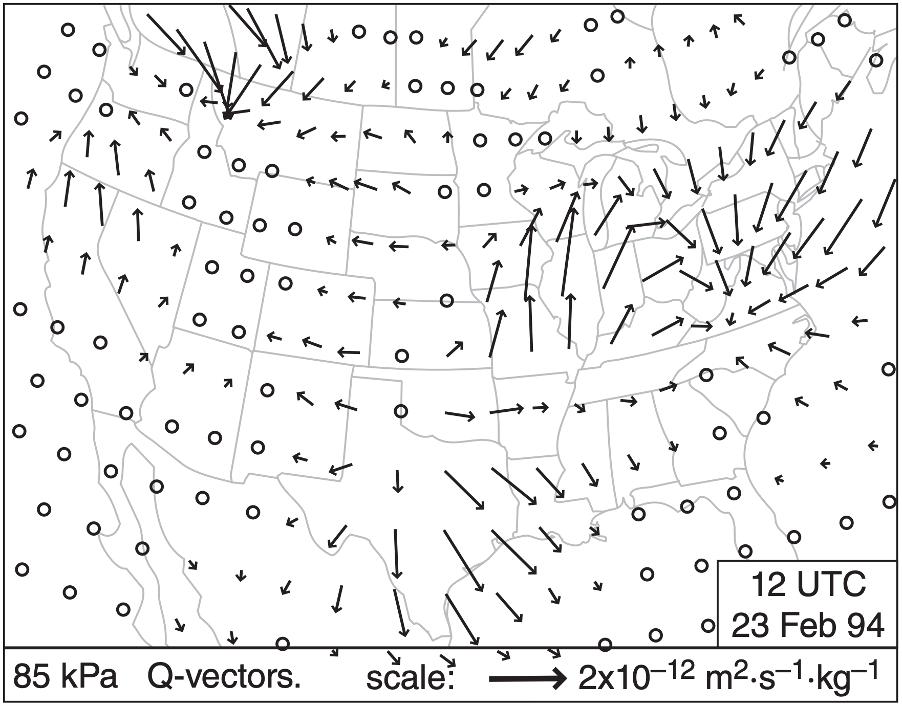
Different locations usually have different Q-vectors, as sketched in Fig. 13.40 for a 1994 event. Interpret Q-vectors on a synoptic weather map as follows:

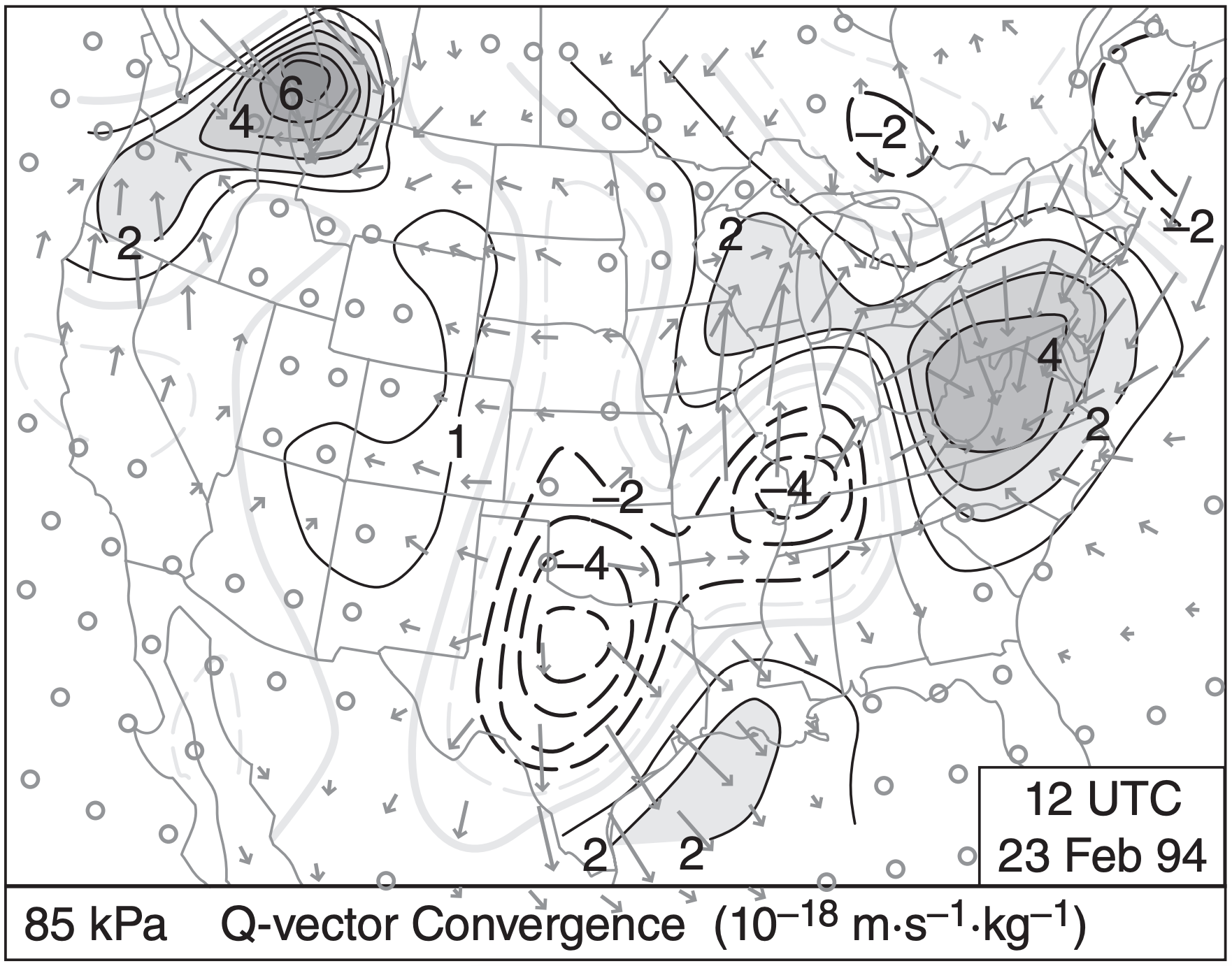
• Updrafts occur where Q-vectors converge. (Fig. 13.41 gives an example for the 1994 event).
• Subsidence (downward motion) occurs where Qvectors diverge.
• Frontogenesis occurs where Q-vectors cross isentropes (lines of constant potential temperature) from cold toward warm.
• Updrafts in the TROWAL region ahead of a warm occluded front occur during cyclolysis where the along-isentrope component of Q-vectors converge.

Using the tricks for visually recognizing patterns of vectors on weather maps (Fig. 13.38b), you can identify by eye regions of convergence and divergence in Fig. 13.40. Or you can let the computer analyze the Q-vectors directly to plot Q-vector convergence and divergence (Fig. 13.41). Although Figs. 13.40 and 13.41 are analysis maps of current weather, you can instead look at Q-vector forecast maps as produced automatically by numerical weather prediction models (see the NWP chapter) to help you forecast regions of updraft, clouds, and precipitation.

Remember that Q-vector convergence indicates regions of likely synoptic-scale upward motion and associated clouds and precipitation. Looking at Fig. 13.41, see a moderate convergence region running from the western Gulf of Mexico up through eastern Louisiana and southern Mississippi. It continues as a weak convergence region across Alabama and Georgia, and then becomes a strong convergence region over West Virginia, Virginia and Maryland. A moderate convergence region extends northwest toward Wisconsin.

This interpretation agrees with the general locations of radar echoes of precipitation for this 1994 event. Note that the frontal locations need not correspond to the precipitation regions. This demonstrates the utility of Q-vectors — even when the updrafts and precipitation are not exactly along a front, you can use Q-vectors to anticipate the bad-weather regions.

Also, along the Texas Gulf coast, the Q-vectors in Fig. 13.40 are crossing the cold front from cold toward warm air. Using the third bullet on the previous page, you can anticipate frontogenesis in this region.

13.5.3.4. Resolving the Geostrophic Paradox

What about the ageostrophic circulations that were missing from the Trenberth omega equation? Fig. 13.41 suggests updrafts at the Q-vector convergence region over the western Gulf of Mexico, and subsidence at the divergence region of central Texas. Due to mass continuity, you can expect an ageostrophic circulation of mid-tropospheric winds from the southeast toward the northwest over the Texas Gulf coast, which connects the up- and down-draft portions of the circulation. This ageostrophic wind moves warm pre-frontal air up over the cold front in a direct circulation (i.e., a circulation where warm air rises and cold air sinks).

But if you had used the 85 kPa height chart to anticipate geostrophic winds over central Texas, you would have expected light winds at 85 kPa from the northwest. These opposing geostrophic and ageostrophic winds agree nicely with the warm-air convergence (creating thunderstorms) for the cold katafront sketch in Fig. 12.16a.

Similarly, over West Virginia and Maryland, Fig. 13.41 shows convergence of Q-vectors at low altitudes, suggesting rising air in that region. This updraft adds air mass to the top of the air column, increasing air pressure in the jet streak right entrance region, and tightening the pressure gradient across the jet entrance. This drives faster geostrophic winds that counteract the advection of slower geostrophic winds in the entrance region. Namely, the ageostrophic winds as diagnosed using Q-vectors help prevent the Geostrophic Paradox (INFO Box).

Sample Application

Discuss the nature of circulations and anticipated frontal and cyclone evolution, given the Q-vector divergence region of southern Illinois and convergence in Maryland & W. Virginia, using Fig. 13.41.

Find the Answer

Given: Q-vector convergence fields.

Discuss: circulations, frontal & cyclone evolution

Exposition: For this 1994 case there is a low center over southern Illinois, right at the location of maximum divergence of Q-vectors in Fig. 13.41. This suggests that: (1) The cyclone is entering the cyclolysis phase of its evolution (synoptic-scale subsidence that opposes any remaining convective updrafts from earlier in the cyclones evolution) as it is steered northeastward toward the Great Lakes by the jet stream. (2) The cyclone will likely shift toward the more favorable updraft region over Maryland. This shift indeed happened.

The absence of Q-vectors crossing the fronts in western Tennessee and Kentucky suggest no frontogenesis there.

Between Maryland and Illinois, we would anticipate a mid-tropospheric ageostrophic wind from the east-northeast. This would connect the updraft region over western Maryland with the downdraft region over southern Illinois. This circulation would move air from the warm-sector of the cyclone to over the low center, helping to feed warm humid air into the cloud shield over and north of the low.

HIGHER MATH • Q-vector Omega Eq.

By considering the added influence of ageostrophic winds, the Q-vector omega equation is:

\(\begin{aligned}\left\{\nabla_{p}^{2}+\frac{f_{0}^{2}}{\sigma} \frac{\partial^{2}}{\partial p^{2}}\right\} \omega=\frac{-2}{\sigma} \cdot\left[\frac{\partial Q_{1}}{\partial x}+\frac{\partial Q_{2}}{\partial y}\right]+\frac{f_{0} \cdot \beta}{\sigma} \frac{\partial V_{g}}{\partial p} -\frac{R / C_{p}}{\sigma \cdot P} \nabla^{2}\left(\Delta Q_{H}\right) \end{aligned}\)

The left side looks identical to the original omega equation (see a previous HIGHER MATH box for an explanation of most symbols). The first term on the right is the convergence of the Q vectors. The second term is small enough to be negligible for synopticscale systems. The last term contributes to updrafts if there is a local maximum of sensible heating ∆Q_H.