20.1: Scientific Basis of Forecasting

20.1.1. The Equations of Motion

Numerical weather forecasts are made by solving Eulerian equations for U, V, W, T, rT, ρ and P.

From the Forces & Winds chapter are forecast equations for the three wind components (U, V, W) (modified from eqs. 10.23a & b, and eq. 10.59):

\begin{align}
\frac{\Delta U}{\Delta t}=-U \frac{\Delta U}{\Delta x}-V \frac{\Delta U}{\Delta y}-W \frac{\Delta U}{\Delta z}
-\frac{1}{\rho} \cdot \frac{\Delta P}{\Delta x}+f_{c} \cdot V-\frac{\Delta F_{z\ turb} (U)}{\Delta z}
\tag{20.1}\end{align}

\begin{align}
\frac{\Delta V}{\Delta t}=-U \frac{\Delta V}{\Delta x}-V & \frac{\Delta V}{\Delta y}-W \frac{\Delta V}{\Delta z}
-\frac{1}{\rho} \cdot \frac{\Delta P}{\Delta y}-f_{c} \cdot U-\frac{\Delta F_{z\ turb}(V)}{\Delta z}
\tag{20.2}\end{align}

\begin{align}
\frac{\Delta W}{\Delta t}=-U \frac{\Delta W}{\Delta x}-V & \frac{\Delta W}{\Delta y}-W \frac{\Delta W}{\Delta z}
-\frac{1}{\rho} \frac{\Delta P^{\prime}}{\Delta z}+\frac{\theta_{v p}-\theta_{v e}}{\bar{T}_{v e}} \cdot|g|-\frac{\Delta F_{z\ t u r b}(W)}{\Delta z}
\tag{20.3}\end{align}

From the Heat Budgets chapter is a forecast equation for temperature T (modified from eq. 3.51):

\begin{align}
\frac{\Delta T}{\Delta t}=-U \frac{\Delta T}{\Delta x}-V \frac{\Delta T}{\Delta y}-W\left[\frac{\Delta T}{\Delta z}+\Gamma_{d}\right]
-\frac{1}{\rho \cdot C_{p}} \frac{\Delta \mathbb{F}_{z\ r a d}^{*}}{\Delta z}+\frac{L_{v}}{C_{p}} \frac{\Delta r_{\text {condensing}}}{\Delta t}-\frac{\Delta F_{z\ t u r b}(\theta)}{\Delta z}
\tag{20.4}\end{align}

From the Water Vapor chapter is a forecast equation (4.44) for total-water mixing ratio r_T in the air:

\begin{align}
\frac{\Delta r_{T}}{\Delta t}=-U \frac{\Delta r_{T}}{\Delta x}-V \frac{\Delta r_{T}}{\Delta y}-W \frac{\Delta r_{T}}{\Delta z}
+\frac{\rho_{L}}{\rho_{d}} \frac{\Delta P r}{\Delta z}-\frac{\Delta F_{z\ turb}\left(r_{T}\right)}{\Delta z}
\tag{20.5}\end{align}

From the Forces & Winds chapter is the continuity equation (10.60) to forecast air density ρ:

\begin{align}\frac{\Delta \rho}{\Delta t}=-U \frac{\Delta \rho}{\Delta x}-V \frac{\Delta \rho}{\Delta y}-W \frac{\Delta \rho}{\Delta z}-\rho\left[\frac{\Delta U}{\Delta x}+\frac{\Delta V}{\Delta y}+\frac{\Delta W}{\Delta z}\right]\tag{20.6}\end{align}

For pressure P, use the equation of state (ideal gas law) from Chapter 1 (eq. 1.23):

\begin{align}P=\rho \cdot \Re_{d} \cdot T_{v}\tag{20.7}\end{align}

INFO • Alternative Vertical Coordinate

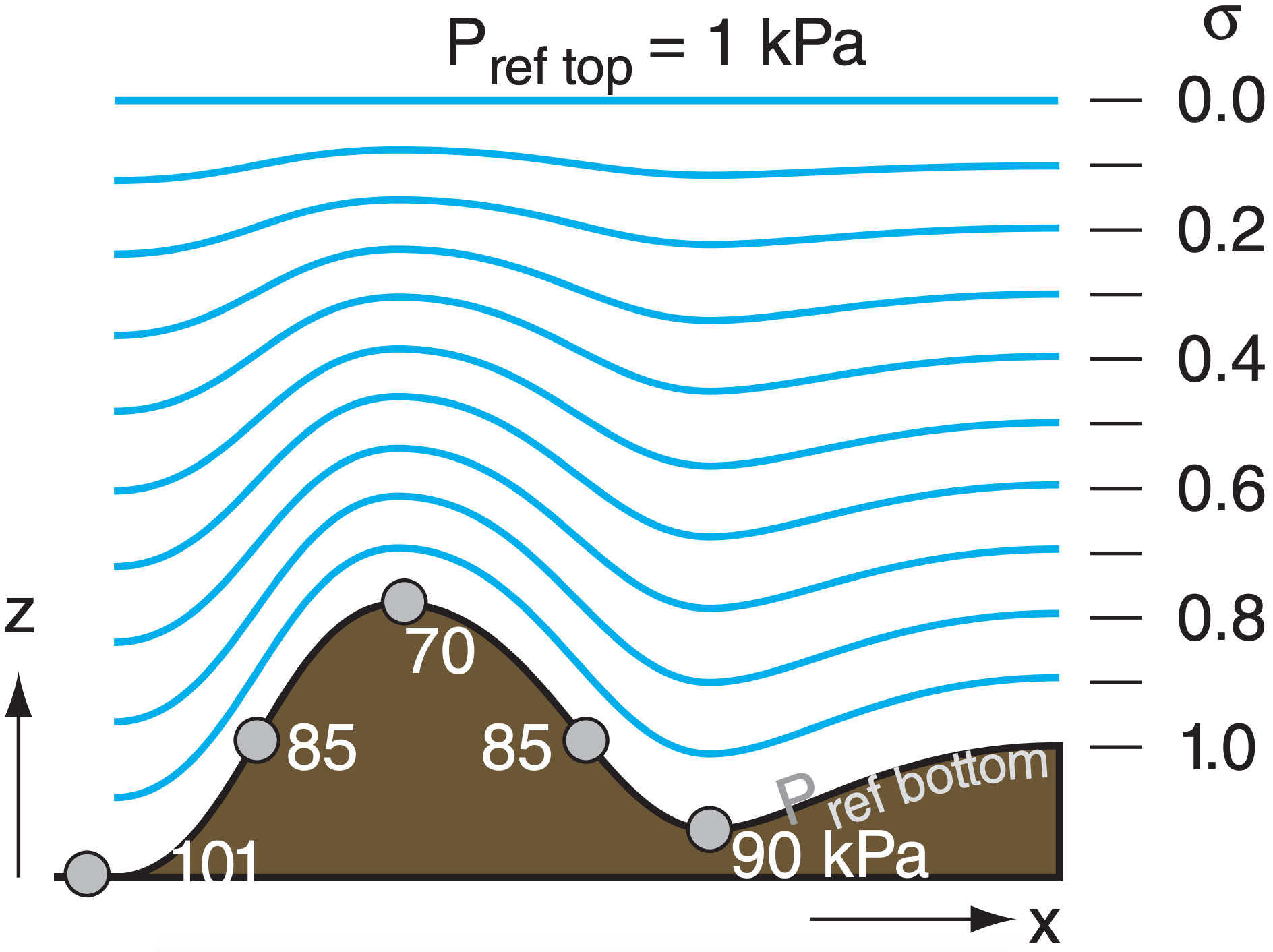
Eqs. (20.1-20.7) use z as a vertical coordinate, where z is height above mean sea level. But local terrain elevations can be higher than sea level. The atmosphere does not exist underground; thus, it makes no sense to solve the meteorological equations of motion at heights below ground level.

To avoid this problem, define a terrain-following coordinate σ (sigma). One definition for σ is based on the hydrostatic pressure P_ref(z) at any height z relative to the hydrostatic pressure difference between the earth’s surface (P_{ref bottom}) and a fixed pressure (P_{ref top}) representing the top of the atmosphere:

\(\ \sigma=\frac{P_{r e f}(z)-P_{r e f\ t o p}}{P_{r e f \ bottom }-P_{r e f\ t o p}}\)

P_{ref bottom} varies in the horizontal due to terrain elevation (see Fig. 20.A) and varies in space and time due to changing surface weather patterns (high- and lowpressure centers). The new vertical coordinate σ varies from 1 at the earth’s surface to 0 at the top of the domain.

The figure below shows how this sigma coordinate varies over a mountain. Hybrid coordinates (Fig. 20.5) are ones that are terrain following near the ground, but constant pressure aloft.

If σ is used as a vertical coordinate, then (U, V) are defined as winds along a σ surface. The vertical advection term in eq. (20.1) changes from W·∆U/∆z to \(\ \dot{\sigma} \cdot \Delta U / \Delta \sigma\), where \(\ \dot{\mathbf{\sigma}}\) is analogous to a vertical velocity, but in sigma coordinates. Similar changes must be made to most of the terms in the equations of motion, which can be numerically solved within the domain of 0 ≤ σ ≤ 1.

Figure 20.A. Vertical cross section through the atmosphere (white) and earth (brown). White numbers represent surface air pressure at the weather stations shown by the grey dots. For the equation above, P_{ref bottom} = 70 kPa at the mountain top, which differs from P_{ref bottom} = 90 kPa in the valley.

Although sigma coordinates avoid the problem of coordinates that go underground, they create problems for advection calculations due to small differences between large terms.

In these seven equations: f_c is Coriolis parameter; P’ is the deviation of pressure from its hydrostatic value; θ_vp and θ_ve are virtual potential temperatures of the air parcel and the surrounding environment;T_ve is virtual temperature of the environment; |g| = 9.8 m s^–2 is the magnitude of gravitational acceleration; Γ_d = 9.8 K km^–1 is the dry adiabatic lapse rate; F*_{z rad} is net radiative flux; L_v ≈ 2.5x10⁶ J kg^–1 is the latent heat of vaporization; C_p ≈ 1004 J·kg^–1·K^–1 is the specific heat of air at constant pressure; ∆r_condensing is the increase in liquid-water mixing ratio associated with water vapor that is condensing; ρ_L ≈ 1000 kg·m^–3 and ρd are the densities of liquid water and dry air; Pr is precipitation rate (m s^–1) of water accumulation in a rain gauge at any height z; ℜ_d = 287 J·kg^–1·K^–1 is the gas constant for dry air; and T_v is the virtual temperature. For more details, see the chapters cited with eqs. (20.1 - 20.7).

Notice the similarities in eqs. (20.1 - 20.6). All have a tendency term (rate of change with time) on the left. All have advection as the first 3 terms on the right. Eqs. (20.1 - 20.5) include a turbulence flux divergence term on the right. The other terms describe the special forcings that apply to individual variables. Sometimes the hydrostatic equation (Chapter 1, eq. 1.25b) is also included in the set of forecast equations:

\(\ \begin{align}\frac{\Delta P_{r e f}}{\Delta z}=-\rho \cdot|g|\tag{20.8}\end{align}\)

to serve as a reference state for the definition of P’ = P – P_ref , as used in eq. (20.3).

Equations (20.1) - (20.7) are the equations of motion. They are also known as the primitive equations, because they forecast fundamental (primitive) variables rather than derived variables such as vorticity. The first six equations are budget equations, because they forecast how variables change in response to inputs and outputs. Namely, the first three equations describe momentum conservation per unit mass of air. Eqs. (20.4 - 20.5) describe heat conservation and moisture conservation per unit mass of air. Eq. (20.6) describes mass conservation.

The first six equations are prognostic (i.e., forecast the change with time), and the seventh (the ideal gas law) is diagnostic (not a function of time). The third equation includes non-hydrostatic processes, the fourth equation includes diabatic processes (non-adiabatic heating), and the sixth equation includes compressible processes.

These equations of motion are nonlinear, because many of the terms in these equations consist of products of two or more dependent variables. Also, they are coupled equations, because each equation contains variables that are forecast or diagnosed from one or more of the other equations. Hence, all 7 equations must be solved together.

Unfortunately, no one has yet succeeded in solving the full governing equations analytically. An analytical solution is itself an algebraic equation or number that can be applied at every location in the atmosphere. For example, the equation y² + 2xy = 8x² has an analytical solution y = 2x, which allows you to find y at any location x.

INFO • Alternative Horizontal Coord.

Spherical Coordinates

For the Cartesian coordinates used in eqs. (20.1- 20.8), the coordinate axes are straight lines. However, on Earth we prefer to define x to follow the Earth’s curvature toward the East, and define y to follow the Earth’s curvature toward the North. If U and V are defined as velocities along these spherical coordinates, then add the following terms (20.1b - 20.3b) to the right sides of momentum eqs. (20.1 - 20.3), respectively:

\begin{align}+\frac{U \cdot V \cdot \tan (\phi)}{R_{o}}-\frac{U \cdot W}{R_{o}}-[2 \cdot \Omega \cdot W \cdot \cos (\phi)]\tag{20.1b}\end{align}

\begin{align}-\frac{U^{2} \cdot \tan (\phi)}{R_{o}}-\frac{V \cdot W}{R_{o}}\tag{20.2b}\end{align}

\begin{align}+\frac{U^{2}+V^{2}}{R_{o}}+[2 \cdot \Omega \cdot U \cdot \cos (\phi)]\tag{20.3b}\end{align}

where R_o ≈ 6371 km is the average Earth radius, ϕ is latitude, and Ω = 0.7292x10^–4 s^–1 is Earth’s rotation rate. The terms containing R_o are called the curvature terms. The terms in square brackets are small components of Coriolis force (see the INFO Box “Coriolis Force in 3-D” from the Forces & Winds chapter).

Map Factors

Suppose we pick (x, y) to represent horizontal coordinates on a map projection, such as shown in the INFO Box on the next page. Let (U, V) be the horizontal components of winds in these (x, y) directions. [Vertical velocity W applies unchanged in the z (up) direction.] One reason why meteorologists use such map projections is to avoid singularities, such as near the Earth’s poles where meridians converge.

The equations of motion can be rewritten for any map projection. For example, eq. (20.1) can be written for a polar stereographic projection as:

\begin{align}
\frac{\Delta U}{\Delta t}=-& m_{0} \cdot U \frac{\Delta U}{\Delta x}-m_{0} \cdot V \frac{\Delta U}{\Delta y}-W \frac{\Delta U}{\Delta z}
-m_{x} \cdot V^{2}+m_{y} \cdot U \cdot V-\frac{U \cdot W}{R_{0}}+[\text { Cor }]
-\frac{m_{0}}{\rho} \cdot \frac{\Delta P}{\Delta x}+f_{c} \cdot V-\frac{\Delta F_{z\ turb}(U)}{\Delta z}
\tag{20.1c}\end{align}

where [Cor] is a 3-D Coriolis term, and the map factors (m) are:

\(\ m_{o}=\frac{1+\sin \left(\phi_{0}\right)}{1+\sin (\phi)}=\frac{L^{2}+x^{2}+y^{2}}{2 \cdot R_{o} \cdot L}\)

and

\(\ m_{x}=x /\left(R_{o} \cdot L\right) \quad, \quad m_{y}=y /\left(R_{o} \cdot L\right)\)

where L = R_o · [1+sin(ϕ_o)], R_o ≈ 6371 km is the average Earth radius, ϕ is latitude, and ϕ_o is the reference latitude for the map projection (see INFO Box).

Thus, the equation has extra terms, and many of the terms are scaled by a map factor. Eqs. (20.2 - 20.6) have similar changes when cast on a map projection.

Sample Application (§)

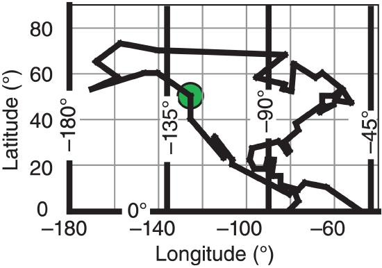
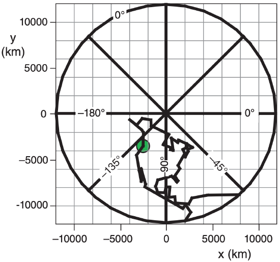
Plot the given coordinates: (a) on a lat-lon grid, and (b) on a polar stereographic grid with ϕ_o = 60°.

Find the Answer

Given: Latitudes (ϕ) & longitudes (λ) of N. America
Each column holds [ϕ(°) λ(°)]. λ is positive eastward
50 -125 40 -125 23 -110 24 -110 30 -115 32 -114 22 -106 20 -106 7 -80 9 -78 4 -76 0 -80 0 -48 10 -63 12 -73	9 -76 11 -84 15 -84 15 -88 22 -87 22 -90 18 -91 18 -96 22 -98 27 -97 30 -85 28 -83 25 -81 26 -80 30 -82 35 -76	38 -77 46 -65 43 -66 46 -60 45 -65 50 -65 50 -60 53 -56 48 -59 47 -52 53 -56 60 -65 58 -68 64 -78 52 -79 53 -83	55 -82 58 -95 68 -82 70 -140 73 -157 65 -168 58 -158 53 -170 60 -146 60 -140 50 -125 0 -90 0 90	0 0 0 180 0 -45 0 135 0 45 0 -135 0 0 0 10 0 20 0 30 0 etc. 0 350 0 360

Hint: In Excel, copy these numbers into 2 long columns: the first for latitudes and the second for longitudes. Leave blank rows in Excel corresponding to the blank lines in the table, to create discontinuous plotted lines.

(a) Lat-Lon Grid:

To save space, only the portion of the grid near North America is plotted.

Fig. 20.B1.

(b) Polar Stereographic Grid:

Hint: In Excel, don’t forget to convert from (°) to (radians).

To demonstrate the Excel calculation for the first coordinate (near Vancouver): ϕ = 50° , λ = –125° : L = (6371 km)·[1 + sin(60°·π/180°)] = 11,888 km.

r = (11888 km)·tan[0.5·(90°– 50°)·π/180°] = 4327 km

x = (4327 km)·cos(–125°·π/180°) = – 2482 km

y = (4327 km)·sin(–125°·π/180°) = – 3545 km

That point is circled in green on the maps above and below.

Fig. 20.B2

INFO • Map Projections

A map displays the 3-D Earth’s surface on a 2-D plane. On maps you can also: (1) create perpendicular (x, y) coordinates; and (2) rewrite the equations of motion within these map coordinates. You can then solve these eqs. to make numerical weather forecasts.

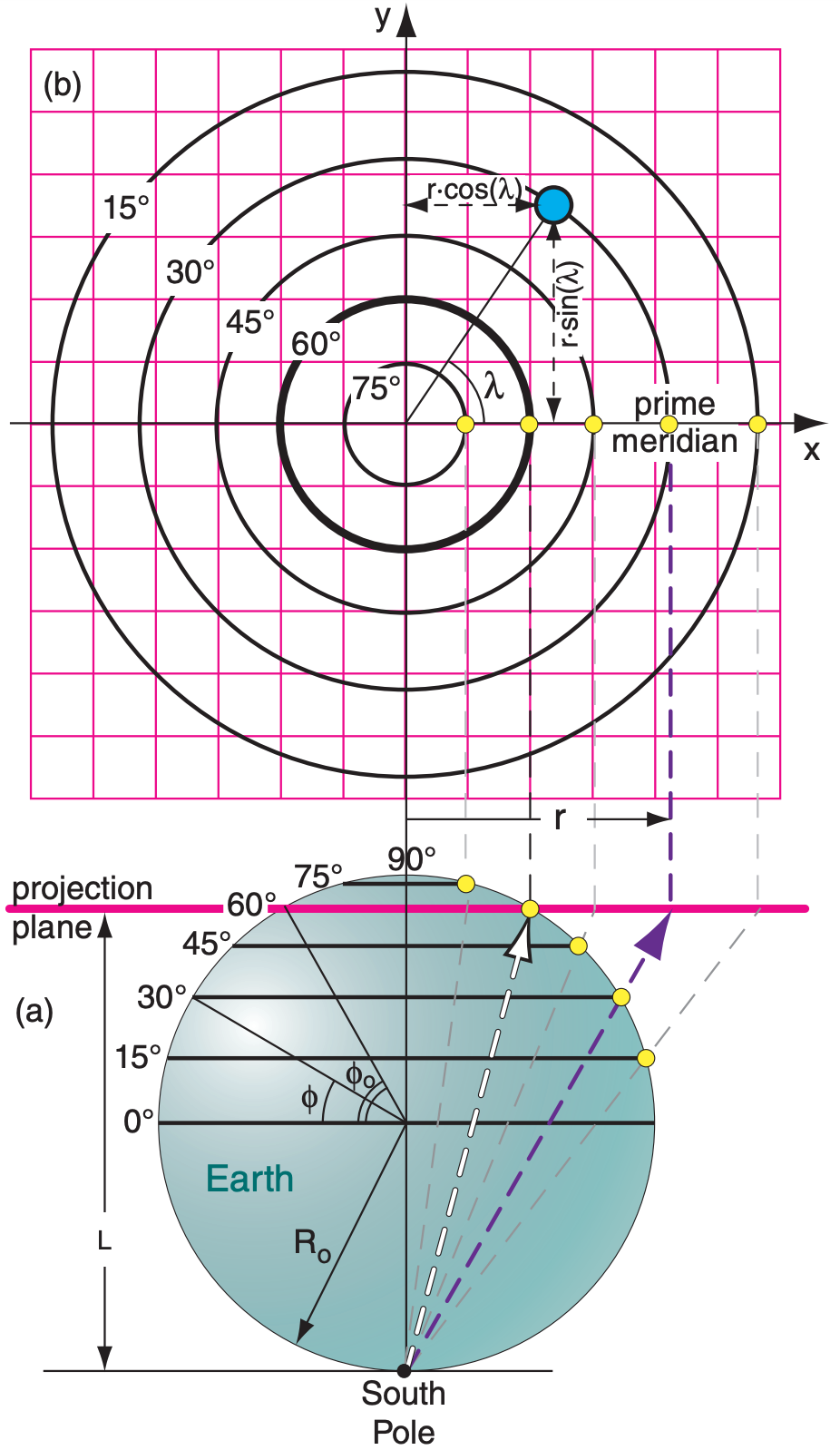
Create a map by projecting the spherical Earth onto a plane (stereographic projection), a cylinder (Mercator projection), or a cone (Lambert projection), where the cylinder and cone can be “unrolled” after the projection to give a flat map. Although other map projections are possible, the 3 listed above are conformal, meaning that the angle between two intersecting curves on the Earth is equal to the angle between the same curves on the map.

For stereographic projections, if the projector is at the North or South Pole, then the result is a polar stereographic projection (Fig. 20.C). For any latitude (ϕ) longitude (λ, positive eastward) coordinates on Earth, the corresponding (x, y) map coordinates are:

\begin{align}x=r \cdot \cos (\lambda), \quad y=r \cdot \sin (\lambda)]\tag{F20.1}\end{align}

\begin{align}r=L \cdot \tan \left[0.5 \cdot\left(90^{\circ}-\phi\right)\right], L=R_{o} \cdot\left[1+\sin \left(\phi_{\mathrm{o}}\right)\right]\tag{F20.2}\end{align}

where R_o = 6371 km = Earth’s radius and ϕ_o is the latitude intersected by the projection plane. The Fig. below has ϕ_o = 60°, but often ϕ_o = 90° is used instead.

Fig. 20.C. Polar stereographic map projection.

20.1.2. Approximate Solutions

To get around this difficulty of no analytical solution, three alternatives are used. One is to find an exact analytical solution to a simplified (approximate) version of the governing equations. A second is to conceive a simplified physical model, for which exact equations can be solved. The third is to find an approximate numerical solution to the full governing equations (the focus of this chapter).

(1) An atmospheric example of the first method is the geostrophic wind, which is an exact solution to a highly simplified equation of motion. This is the case of steady-state (equilibrium) winds above the boundary layer where friction can be neglected, and for regions where the isobars are nearly straight.

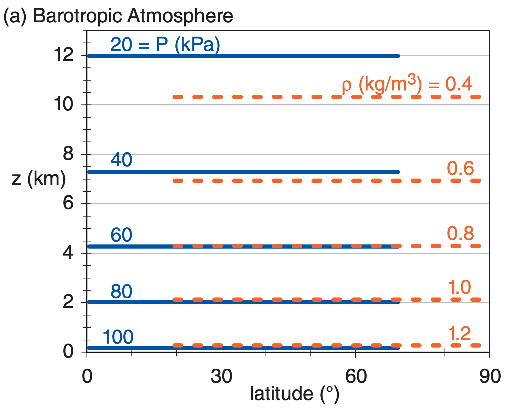
(2) Early numerical weather prediction (NWP) efforts used the 2^nd method, because of the limited power of early computers. Rossby derived simplified equations by modeling the atmosphere as if it were one layer of water surrounding the Earth. Charney, von Neumann, and others extended this work and wrote a program for a one-layer barotropic atmosphere (Fig. 20.2a) for the ENIAC computer in 1950. These earliest programs forecasted only vorticity and geopotential height at 50 kPa.

Figure 20.2 (a) Barotropic idealization, based on the standard atmosphere from Chapter 1. (b) Baroclinic example, based on data from the General Circulation chapter. P is pressure, ρ is density, and z is height.

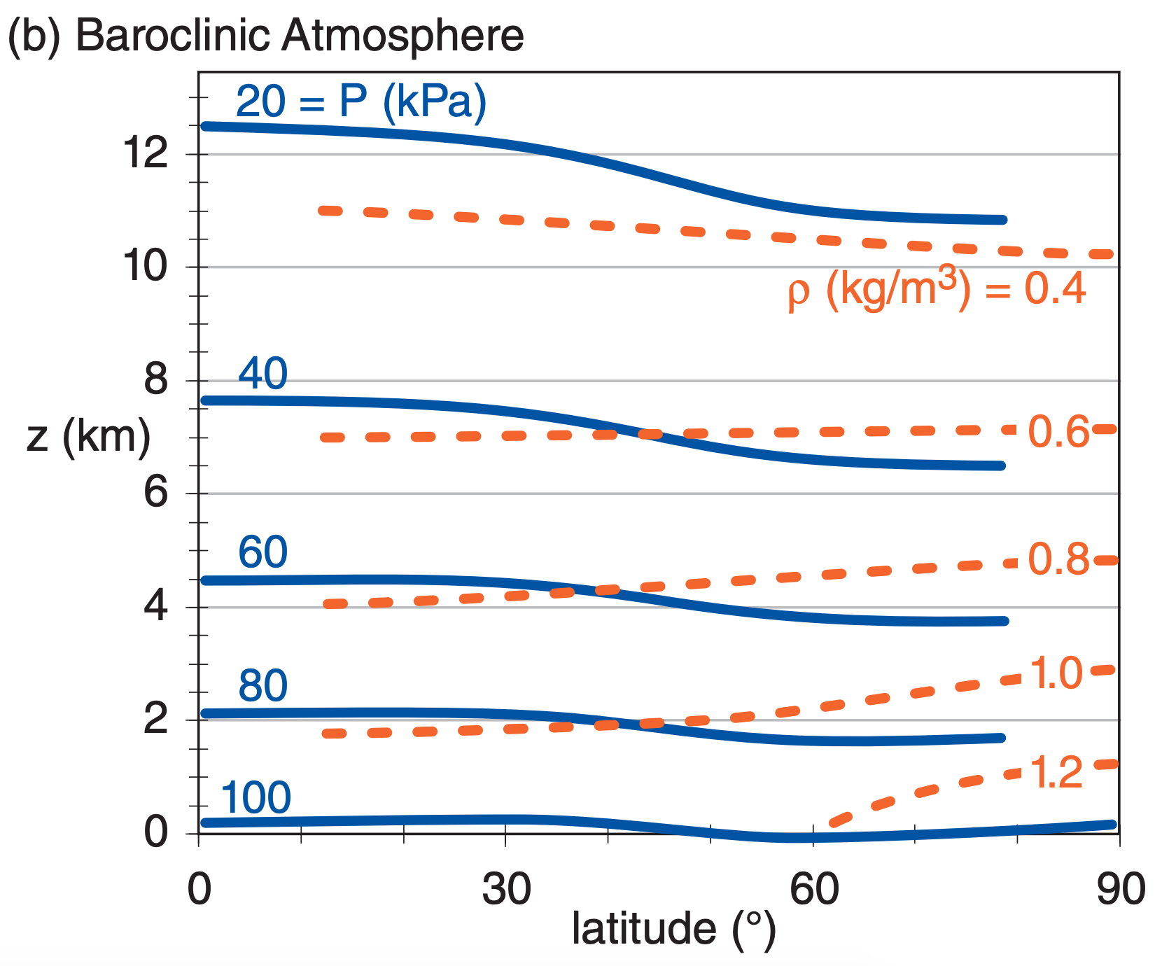
(3) Modern NWP uses the third method. Here, the full primitive equations are solved using finite-difference approximations for full baroclinic scenarios (Fig. 20.2b), but only at discrete locations called grid points. Usually these grid points are at regularly-spaced intervals on a map, rather than at each city or town.

INFO • Barotropic vs. Baroclinic

In a barotropic atmosphere (Fig. 20.2a), the isobars (lines of equal pressure) do not cross the isopycnics (lines of equal density). This would occur for a situation where there are no variations of temperature in the horizontal. Hence, there could be no thermal-wind effect.

In a baroclinic atmosphere (Fig. 20.2b), isobars can cross isopycnics. Horizontal temperature gradients contribute to the tilt of the isopycnics. These temperature gradients also cause changing horizontal pressure gradients with increasing altitude, according to the thermal-wind effect.

The real atmosphere is baroclinic, due to differential heating by the sun (see the General Circulation chapter). In a baroclinic atmosphere, potential energy associated with temperature gradients can be converted into the kinetic energy of winds.

20.1.3. Dynamics, Physics and Numerics

If computers had infinite power, then we could: forecast the movement of every air molecule; forecast the growth of each snowflake and cloud droplet; precisely describe each turbulent eddy; consider atmospheric interaction with each tree leaf and blade of grass; diagnose the absorption of radiation for an infinite number of infinitesimally fine spectral bands; account for every change in terrain elevation; and could even include the movement and activities of each human as they affect the atmosphere. But it might be a few years before we can do that. At present, we must make compromises to our description of the atmosphere.

Numerics: The main compromise is the process of discretization, where:

(1) we split the continuum of space into a finite number of small volumes called grid cells (Fig. 20.3a), within which we forecast average conditions;

(2) we approximate the smooth progression of time with finite time steps; and

(3) we replace the elegant equations of motion with numerical approximations.

Figure 20.3 (a) The forecast domain (the portion of atmosphere we wish to forecast) is split into discrete grid cells, such as the cyan shaded one. The 3-D grid cells are relatively thin, with vertical sizes on the order of tens of meters, and horizontal sizes of tens of kilometers.

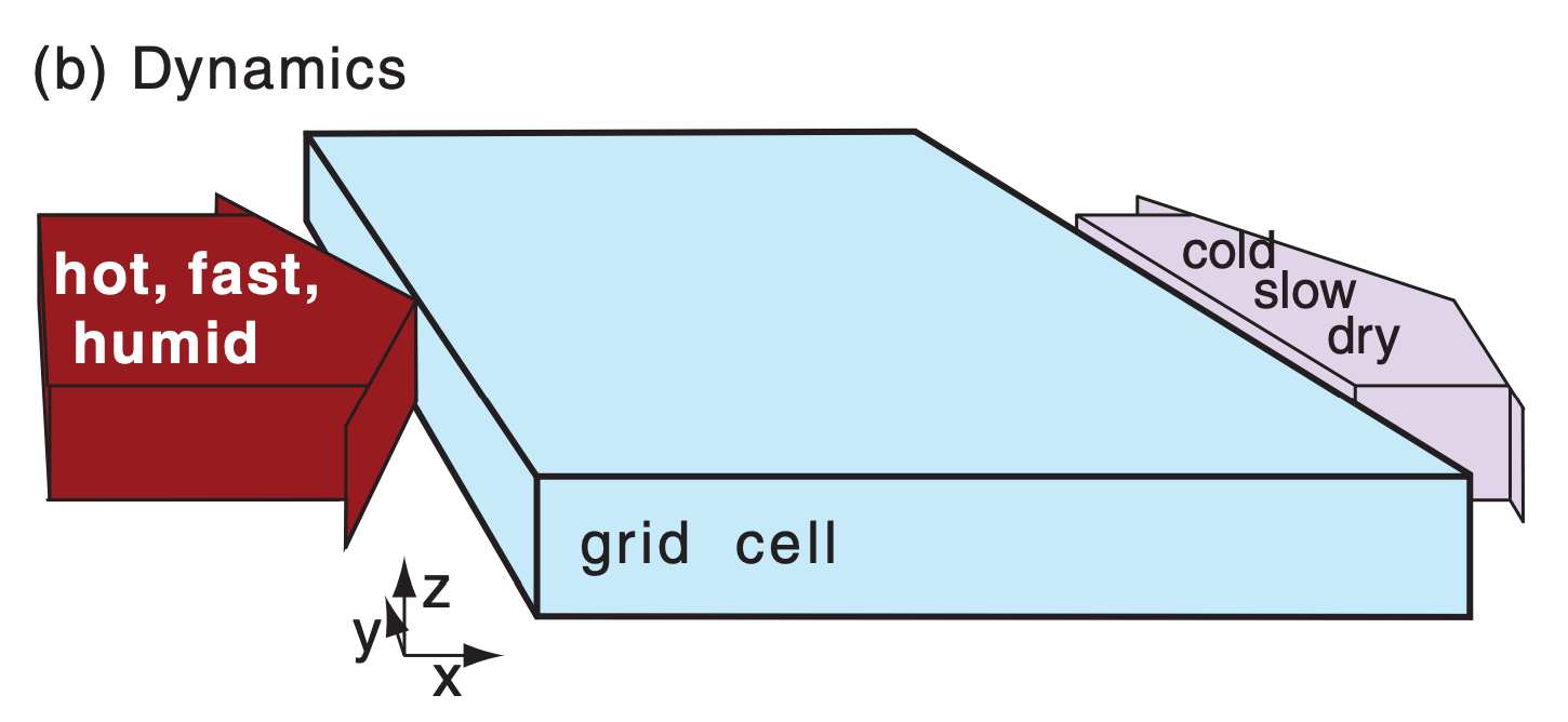
(b) Enlargement of the shaded grid cell, illustrating one dynamics process (advection in the x-direction). Namely, the resolved U wind is blowing in hot, fast, humid air from the upwind neighboring grid cell, and is blowing out colder, slower, drier air into the downwind neighboring cell. Simultaneously, advection could be occurring by the V and W components of wind (not shown). Not shown are other resolved forcings, such as Coriolis and pressure-gradient forces.

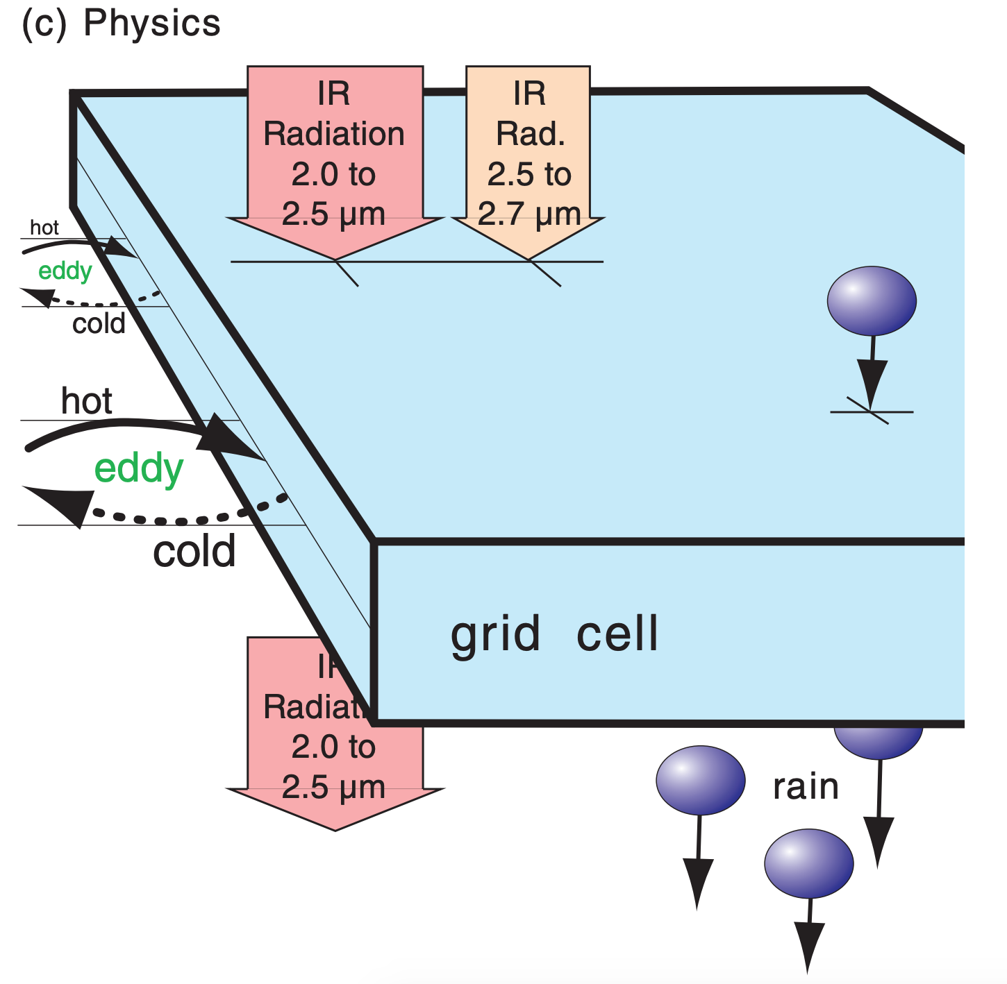
(c) Further enlargement, illustrating physics such as turbulence, radiation, and precipitation. Turbulence is causing a net heat flux into the left side of the grid cell in this example, even though the turbulence has no net wind (i.e., the wind-gust arrows moving air into the grid cell are balanced by gusts moving the same amount of air out of the grid cell). Two of the many radiation bands are shown, where infrared (IR) wavelengths in the 2.0 to 2.5 µm “window” band shine through the grid cell, while wavelengths in the 2.5 to 2.7 µm band are absorbed by water vapor and carbon dioxide (see the Satellites & Radar chapter), causing warming in the grid cell. Some liquid water is falling into the top of the grid cell from the cell above, but even more is falling out the bottom into the grid cell below, suggesting a removal of water and net latent heating due to condensation.

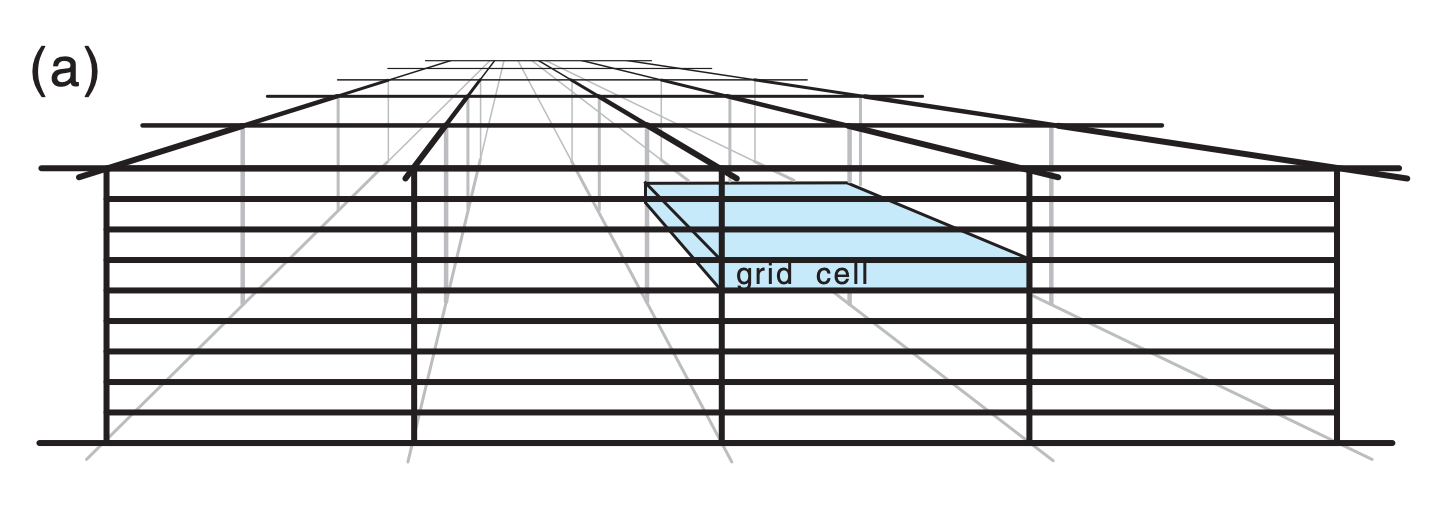
These topics are generically known as numerics, as will be discussed in detail later. Numerics also include the domain being forecast, the mapping and coordinate systems, and the representation of data.

The word “dynamics” refers to the governing equations. It applies to only the resolved portions of motions, thermodynamic states, and moisture states (Fig. 20.3b) for the particular discretization used. A variable or process is said to be resolved if it can be represented by the average state within a grid cell. The dynamics described by eqs. (20.1 - 20.7) depend on sums, differences, and products of these resolved grid-cell average values.

The word “physics” refers to other processes (Fig. 20.3c and Table 20-1) that:

(1) are not forecast by the equations of motion; or

(2) are not well understood even though their effects can be measured; or

(3) involve motions or particles that are too small to resolve (called subgrid scale); or

(4) have components that are too numerous (e.g., individual cloud droplets or radiation bands); or

(5) are too complicated to compute in finite time. However, unresolved processes can combine to produce resolved forecast effects. Because we cannot neglect them, we parameterize them instead.

A parameterization is a physical or statistical approximation to a physical process by one or more known terms or factors. Parameterization rules are given in an “A SCIENTIFIC PERSPECTIVE” box in the Atmos. Boundary Layer chapter. In NWP, the “knowns” are the resolved state variables in the grid cells, and any imposed boundary conditions such as solar radiation, surface topography, land use, ice coverage, etc. Empirically estimated factors called parameters tie the knowns to the approximated physics.

Because parameterizations are only approximations, no single parameterization is perfectly correct. Different scientists might propose different parameterizations for the same physical phenomenon. Different parameterizations might perform better for different weather situations.

Sample Application

Suppose subgrid-scale cloud coverage C is parameterized by

C = 0	for RH ≤ RHo
C = [(RH – RHo) / (1 – RHo)]^2	for RHo ≤ RH < 1
C = 1	for RH ≥ 1

RH is the grid-cell average relative humidity. Parameter RH_o ≈ 0.8 for low and high clouds, and RH_o ≈ 0.65 for mid-level cloud. Plot parameterized cloud coverage vs. resolved relative humidity

Find the Answer

Given: info above

Find: C vs. RH

Spreadsheet solution is graphed at right. Thin cyan curve: mid-level clouds.

Thick green curve: low and high clouds.

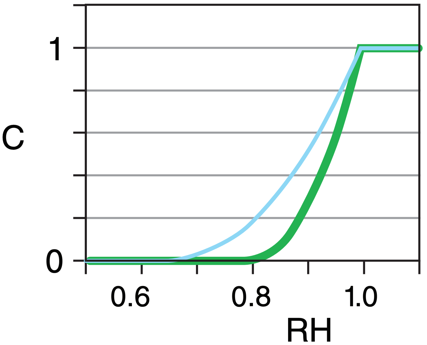
Check: Coverage bounded between clear & overcast.

Exposition: Partial cloud coverage is important for computing how much radiation reaches the ground.

Table 20-1. Some physics parameterizations in NWP
Process	Approximation Methods
Cloud Coverage	• Subgrid-scale cloud coverage as a function of resolved relative humidity. Affects the radiation budget.
Precipitation & Cloud Microphysics	Considers conversions between water vapor, cloud ice, snow, cloud water, rain water, and graupel + hail. Affects large-scale condensation, latent heating, and precipitation based on resolved supersaturation. Methods: • bulk (assumes a size distribution of hydrometeors); or • bin (separate forecasts for each subrange of hydrometeor sizes).
Deep Convection	• Approximations for cumuliform clouds (including thunderstorms) that are narrower than grid-cell width but which span many grid layers in the vertical (i.e., are unresolved in the horizontal but resolved in the vertical), as function of moisture, stability and winds. Affects vertical mixing, precipitation, latent heating, & cloud coverage.
Radiation	• Impose solar radiation based on Earth’s orbit & solar emissions. Include absorption, scattering, & reflection from clouds, aerosols and the surface. • Divide IR radiation spectrum into small number of wide wavelength bands, and track up- and down-welling radiation in each band as absorbed and emitted from/to each grid layer. Affects heating of air & Earth’s surface.
Turbulence	Subgrid turbulence intensity as function of resolved winds and buoyancy. Fluxes of heat, moisture, momentum as function of turbulence and resolved temperature, water, & winds. Methods: • local down-gradient eddy diffusivity; • higher-order local closure; or • nonlocal (transilient turb.) mixing.
Atmospheric Boundary Layer (ABL)	Vertical profiles of temperature, humidity, and wind as a function of resolved state and turbulence, based on forecasts of ABL depth. Methods: • bulk; • similarity theory.
Surface	• Use albedo, roughness, etc. from statistical average of varied land use. • Snow cover, vegetation greenness, etc. based on resolved heat & water budget.
Sub-surface heat & water	• Use climatological average. Or forecast heat conduction & water flow in rivers, lakes, glaciers, subsurface, etc.
Mountainwave Drag	• Vertical momentum flux as function of resolved topography, winds and static stability

20.1.4. Models

The computer code that incorporates one particular set of dynamical equations, numerical approximations, and physical parameterizations is called a numerical model or NWP model. People developing these extremely large sets of computer code are called modelers. It typically takes teams of modelers (meteorologists, physicists, chemists, and computer scientists) several years to develop a new numerical weather model.

Different forecast centers develop different numerical models containing different dynamics, physics and numerics. These models are given names and acronyms, such as the Integrated Forecast System (IFS), Action de Recherche Petite Echelle Grande Echelle (ARPEGE) model, the Unified Model (UM), Weather Research and Forecasting (WRF) model, the Finite Volume - version 3 (FV3) model (see Fig. 20.4c), the Global Environmental Multiscale (GEM) model, the Global Forecast System (GFS), and many more. Different models give slightly different forecasts.