18.4: Temperature

The capping inversion traps in the ABL any heating and water evaporation from the surface. As a result, heat accumulates within the ABL during daytime, or whenever the surface is warmer than the air. Cooling (actually, heat loss) accumulates during nighttime, or whenever the surface is colder than the air. Thus, the temperature structure of the ABL depends on the accumulated heating or cooling.

18.4.1. Cumulative Heating or Cooling

Figure 18.10 Idealization of the heat flux curve over land during fair weather, from Fig. 3.9 of the Heat chapter. Pink shading shows total accumulated heating during the day, while the magenta hatched region shows the portion of heating accumulated up to time t₁ after heating started. Blue shading shows total accumulated cooling during the night.

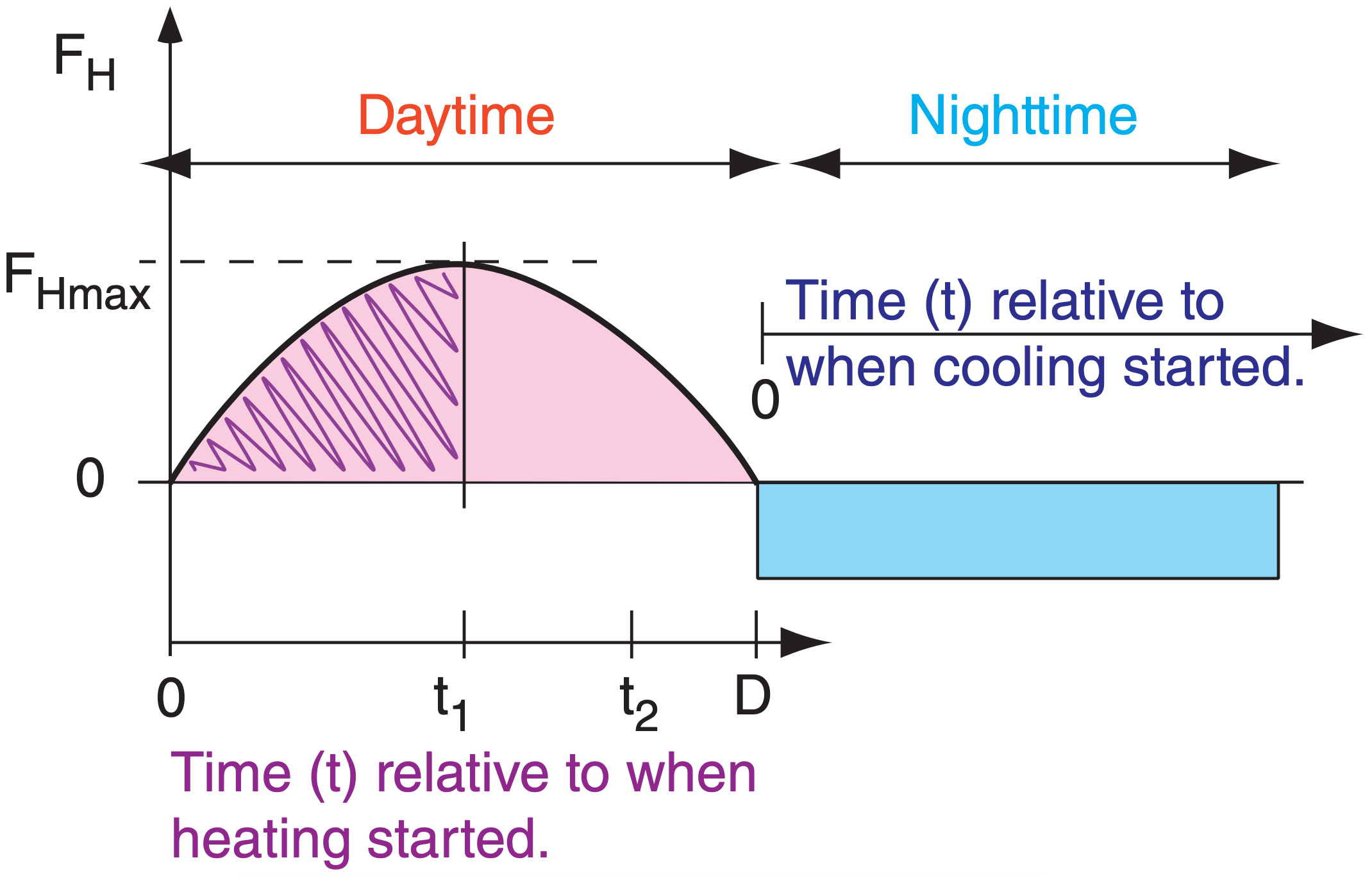
The cumulative effect of surface heating and cooling on ABL evolution is more important than the instantaneous heat flux. This cumulative heating or cooling QA equals the area under the curve of heat flux vs. time (Fig. 18.10). We will examine cumulative nighttime cooling separately from cumulative daytime heating.

18.4.1.1. Nighttime

During clear nights over land, heat flux from the air to the cold surface is relatively constant with time (dark shaded portion of Fig. 18.10) due to persistent infrared radiation from the ground to space. If we define t as the time since cooling began, then the accumulated cooling per unit surface area is:

\(\ \begin{align} Q_{A}=\mathbb{F}_{H} \text { night } \cdot t\tag{18.1a}\end{align}\)

For night, Q_A is a negative number because F_H is negative for cooling. Q_A has units of J m^–2.

Dividing eq. (18.1a) by air density and specific heat (ρ_air·C_p) gives the kinematic form

\(\ \begin{align} Q_{A k}=F_{H \text { night }} \cdot t\tag{18.1b}\end{align}\)

where Q_Ak has units of K·m.

For a night with variable cloudiness that causes a variable surface heat flux (see the Solar & IR Radiation chapter), use the average value of F_H or F_H.

HIGHER MATH • Cumulative Heating

Derivation of Daytime Cumulative Heating

Assume that the kinematic heat flux is approximately sinusoidal with time:

\(\ F_{H}=F_{H \max } \cdot \sin (\pi \cdot t / D)\)

with t and D defined as in Fig. 18.10 for daytime. Integrating from time t = 0 to arbitrary time t :

\(\ Q_{A k}=\int_{t^{\prime}=0}^{t} F_{H} \mathrm{d} t^{\prime}=F_{H \max } \cdot \int_{t^{\prime}=0}^{t} \sin \left(\pi \cdot t^{\prime} / D\right) \mathrm{d} t^{\prime}\)

where t’ is a dummy variable of integration.

From a table of integrals, we find that:

\(\ \int \sin (a \cdot x)=-(1 / a) \cdot \cos (a \cdot x)\)

Thus, the previous equation integrates to:

\(Q_{A k}=\left.\frac{-F_{H \max } \cdot D}{\pi} \cdot \cos \left(\frac{\pi \cdot t}{D}\right)\right|_{0} ^{t}\)

Plugging in the two limits gives:

\(\ Q_{A k}=\frac{-F_{H \max } \cdot D}{\pi} \cdot\left[\cos \left(\frac{\pi \cdot t}{D}\right)-\cos (0)\right]\)

But the cos(0) = 1, giving the final answer (eq. 18.2b):

\(\ Q_{A k}=\frac{F_{H \max } \cdot D}{\pi} \cdot\left[1-\cos \left(\frac{\pi \cdot t}{D}\right)\right]\)

18.4.1.2. Daytime

On clear days, the nearly sinusoidal variation of solar elevation and downwelling solar radiation (Fig. 2.13 in the Solar & IR Radiation chapter) causes nearly sinusoidal variation of surface net heat flux (Fig. 3.9 in the Heat chapter). Let t be the time since F_H becomes positive in the morning, D be the total duration of positive heat flux, and F_{H max} be the peak value of heat flux (Fig. 18.10). These values can be found from data such as in Fig. 3.9. The accumulated daytime heating per unit surface area (units of J m^–2) is:

\(\ \begin{align}Q_{A}=\frac{\mathbb{F}_{H \max } \cdot D}{\pi} \cdot\left[1-\cos \left(\frac{\pi \cdot t}{D}\right)\right]\tag{18.2a}\end{align}\)

In kinematic form (units of K·m), this equation is

\(\ \begin{align}Q_{A k}=\frac{F_{H \max } \cdot D}{\pi} \cdot\left[1-\cos \left(\frac{\pi \cdot t}{D}\right)\right]\tag{18.2b}\end{align}\)

Sample Application

Use Fig. 3.9 from the Heat chapter to estimate the accumulated heating and cooling in kinematic form over the whole day and whole night.

Find the Answer

By eye from Fig. 3.9:

Day: F_{H max} ≈ 150 W·m^–2 , D = 8 h

Night: F_{H night} ≈ –50 W·m^–2 (averaged)

Given: Day: t = D = 8 h = 28800. s

Night: t = 24h – D = 16 h = 57600. s

Find: Q_Ak = ? K·m for day and for night

First convert fluxes to kinematic form by dividing by ρ_air·C_p :

F_{H max} = F_{H max}/ ρ_air·C_p

= (150 W·m^–2 ) / [1231(W·m^–2 )/(K·m s^–1)] = 0.122 K·m s^–1

F_{H night} = (–50W·m^–2)/[1231(W·m^–2)/(K·m s^–1)] = –0.041 K·m s^–1

Day: use eq. (18.2b):

\(\ Q_{A k}=\frac{(0.122 \mathrm{K} \cdot \mathrm{m} / \mathrm{s}) \cdot(28800 \mathrm{s})}{3.14159} \cdot[1-\cos (\pi)]\)

= 2237 K·m

Night: use eq. (18.1b):

Q_Ak = ( –0.041 K·m s^–1)·(57600. s) = –2362 K·m

Check: Units OK. Physics OK.

Exposition: The heating and cooling are nearly equal for this example, implying that the daily average temperature is fairly steady.

18.4.2. Temperature-Profile Evolution

18.4.2.1. Idealized Evolution

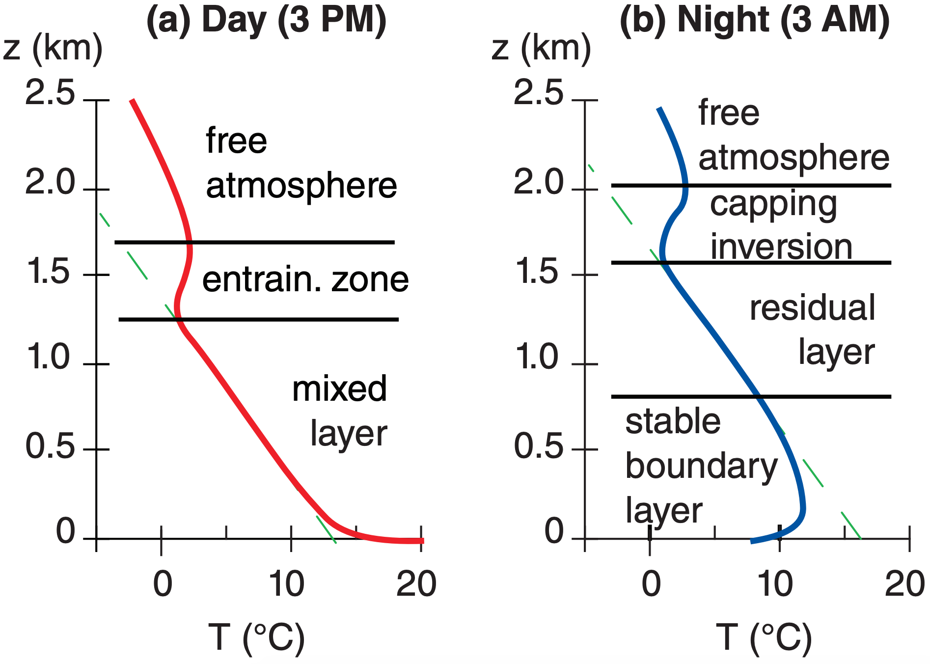
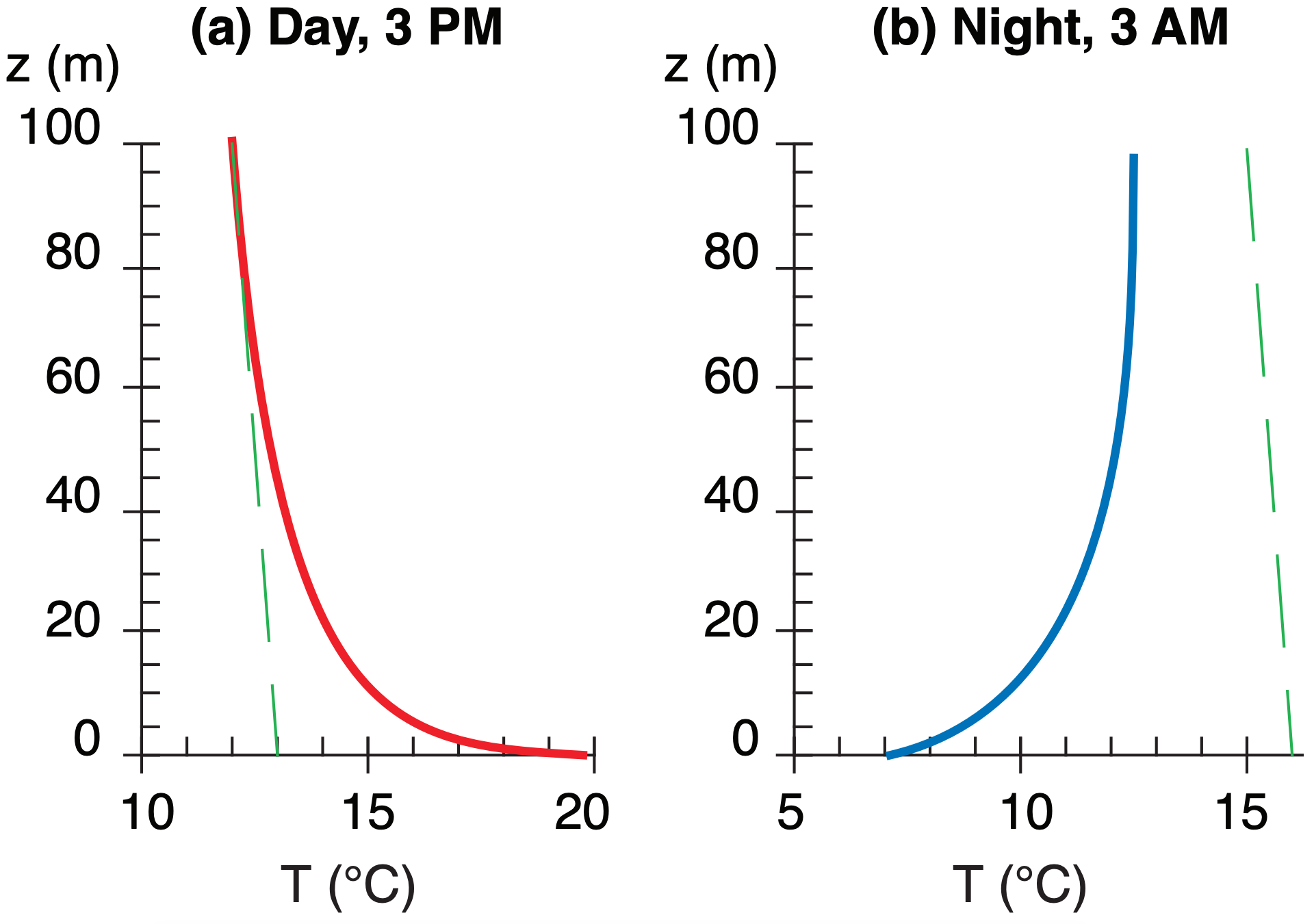
A typical afternoon temperature profile is plotted in Fig. 18.11a. During the daytime, the environmental lapse rate in the mixed layer is nearly adiabatic. The unstable surface layer (plotted but not labeled in Fig. 18.11) is in the bottom part of the mixed layer. Warm blobs of air called thermals rise from this surface layer up through the mixed layer, until they hit the temperature inversion in the entrainment zone. Fig. 18.12a shows a closer view of the surface layer (bottom 5 - 10% of the ABL).

These thermal circulations create strong turbulence and cause pollutants, potential temperature, and moisture to be well mixed in the vertical (hence the name mixed layer). The whole mixed layer, surface layer, and bottom portion of the entrainment zone are statically unstable.

In the entrainment zone, free-atmosphere air is incorporated or entrained into the mixed layer, causing the mixed-layer depth to increase during the day. Pollutants trapped in the mixed layer cannot escape through the EZ, although cleaner, drier free atmosphere air is entrained into the mixed layer. Thus, the EZ is a one-way valve.

At night, the bottom of the mixed layer becomes chilled by contact with the radiatively-cooled ground. The result is a stable ABL. The bottom portion of this stable ABL is the surface layer (again not labeled in Fig. 18.11b, but sketched in Fig. 18.12b).

Above the stable ABL is the residual layer. It has not felt the cooling from the ground, and hence retains the adiabatic lapse rate from the mixed layer of the previous day. Above that is the capping temperature inversion, which is the non-turbulent remnant of the entrainment zone.

Figure 18.11 Examples of boundary-layer temperature profiles during (a) day and (b) night during fair weather over land. The dashed green line indicates the diabatic lapse rate. The heights shown here are illustrative only. In the real ABL the heights can be greater or smaller, depending on location, time, and season.

Figure 18.12 Examples of surface-layer temperature profiles during (a) day & (b) night. The dashed green line shows the adiabatic lapse rate. Again, heights are illustrative only. Actual heights might differ.

18.4.2.2. Seasonal Differences

Figure 18.13 Evolution of potential temperature θ profiles for fair weather over land. Curves are labeled with local time in hours. The summer nighttime curves begin at 18 h local time, which roughly corresponds to the final sounding from the previous day. Winter has shorter daylight hours, so the evening transition occurs at 16 h local time, in this midlatitude idealization.

Figure 18.14 Daily evolution of boundary-layer structure for summer and winter, for fair weather over land. CI = Capping Inversion. Shading indicates static stability: tan = unstable, green = neutral (as in the RL), darker blues = stronger static stabilities.

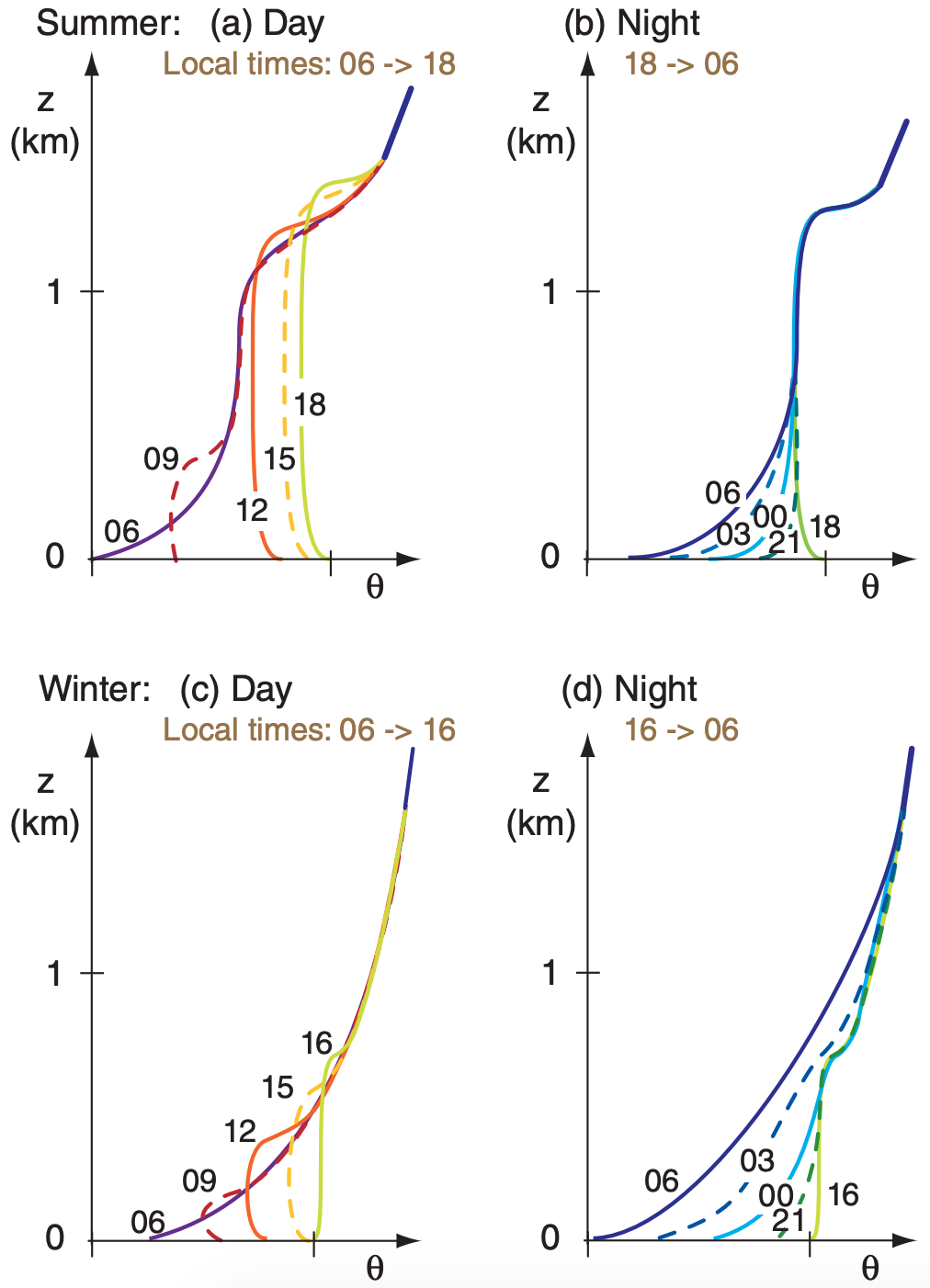
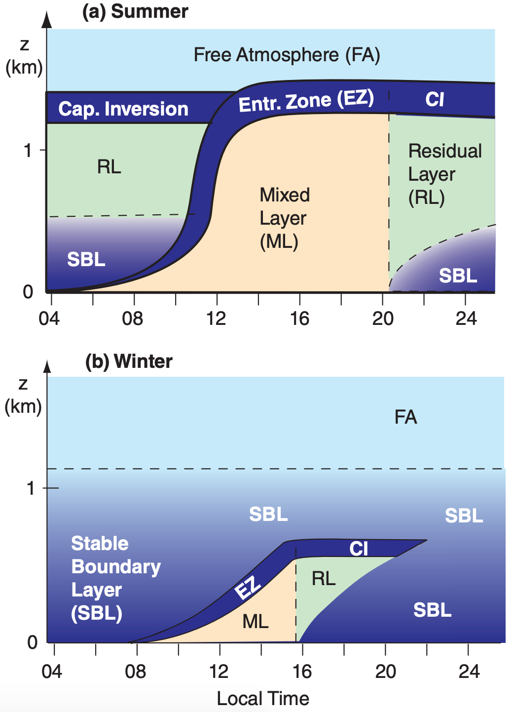
During summer at mid- and high-latitudes, days are longer than nights, allowing more heating to occur during day than cooling at night for fair weather over land. This causes net heating over a 24-h period, as illustrated in Figs. 18.13 a & b. The convective mixed layer starts shallow in the morning, but rapidly grows through the residual layer. In the afternoon, it continues to rise slowly into the free atmosphere. If the air contains sufficient moisture, cumuliform clouds can exist. At night, cooling creates a shallow stable ABL near the ground, but leaves a thick residual layer above it.

During winter at mid- and high-latitudes, more cooling occurs during the long nights than heating during the short days, in fair weather. Stable ABLs dominate over land, and there is net temperature decrease over 24 hours (Figs. 18.13 c & d). Any non-frontal clouds present are typically stratiform or fog. Any residual layer that forms early in the night is quickly consumed by the growing stable ABL.

Fig. 18.14 shows the corresponding structure of the ABL. Although both the mixed layer and residual layer have nearly adiabatic temperature profiles, the mixed layer is nonlocally unstable, while the residual layer is neutral. This difference causes pollutants to disperse at different rates in those two regions.

If the wind moves ABL air over surfaces of different temperatures, then ABL structures can evolve in space, rather than in time. For example, suppose the numbers along the abscissa in Fig. 18.14b represent distance x (km), with wind blowing from left to right over a lake spanning 8 ≤ x ≤ 16 km. The ABL structure in Fig. 18.14b could occur at midnight in mid-latitude winter for air blowing over snow-covered ground, except for the unfrozen lake in the center. If the lake is warmer than the air, it will create a mixed layer that grows as the air advects across the lake.

Don’t be lulled into thinking the ABL evolves the same way at every location or at similar times. The most important factor is the temperature difference between the surface and the air. If the surface is warmer, a mixed layer will develop regardless of the time of day. Similarly, colder surfaces will create stable ABLs.

18.4.3. Stable ABL Temperature

Stable ABLs are quite complex. Turbulence can be intermittent, and coupling of air to the ground can be quite weak. In addition, any slope of the ground causes the cold air to drain downhill. Cold, downslope winds are called katabatic winds, as discussed in the Regional Winds chapter.

Figure 18.15 Idealized exponential-shaped potential temperature profile in the stable (nighttime) boundary layer.

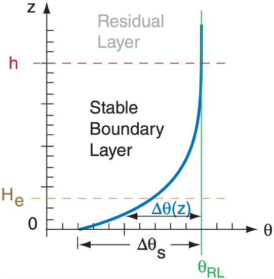
For a simplified case of a turbulent, stable ABL over a flat surface during light winds, the potential temperature profile is approximately exponential with height (Fig. 18.15):

\(\ \begin{align} \Delta \theta(z)=\Delta \theta_{s} \cdot e^{-z / H_{e}}\end{align}\)

where ∆θ(z) = θ(z) – θ_RL is the potential temperature difference between the air at height z and the air in the residual layer. ∆θ(z) is negative.

The value of this difference near the ground is defined to be ∆θ_s = ∆θ(z=0), and is sometimes called the strength of the stable ABL. H_e is an e-folding height for the exponential curve. The actual depth h of the stable ABL is roughly h = 5·H_e.

Depth and strength of the stable ABL grow as the cumulative cooling Q_Ak increases with time:

\(\ \begin{align} H_{e} \approx a \cdot M_{R L}^{3 / 4} \cdot t^{1 / 2}\tag{18.4}\end{align}\)

\(\ \begin{align}\Delta \theta_{S}=\frac{Q_{A k}}{H_{e}}\tag{18.5}\end{align}\)

where a = 0.15 m^1/4 ·s^1/4 for flow over a flat prairie, and where MRL is the wind speed in the residual layer. Because the cumulative cooling is proportional to time, both the depth 5·H_e and strength ∆θ_s of the stable ABL increase with the square root of time. Thus, the fast growth rate of the SBL early in the evening decreases to a much slower growth rate by the end of the night.

Sample Application (§)

Estimate the potential temperature profile at the end of a 12-hour night for two cases: windy (10 m s^–1) and less windy (5 m s^–1). Assume Q_Ak = –1000 K·m.

Find the Answer

Given: Q_Ak = –1000 K·m, t = 12 h

(a) M_RL = 10 m s^–1, (b) M_RL = 5 m s^–1

Find: θ vs. z

Assume: flat prairie. To plot profile, need H_e & ∆θ_s.

Use eq. (18.4):

\(\ H_{e} \approx\left(0.15 \mathrm{m}^{1 / 4} \cdot \mathrm{s}^{1 / 4}\right) \cdot\left(10 \mathrm{m} \cdot \mathrm{s}^{-1}\right)^{3 / 4} \cdot(43200 \mathrm{s})^{1 / 2}\)

(a) H_e = 175 m

\(\ H_{e} \approx\left(0.15 \mathrm{m}^{1 / 4} \cdot \mathrm{s}^{1 / 4}\right) \cdot\left(5 \mathrm{m} \cdot \mathrm{s}^{-1}\right)^{3 / 4} \cdot(43200 \mathrm{s})^{1 / 2}\)

(b) H_e = 104 m

Use eq. (18.5):

(a) ∆θ_s = (–1000K·m)/(175) = –5.71 °C

(b) ∆θ_s = (–1000K·m)/(104) = –9.62 °C

Use eq. (18.3) in a spreadsheet to compute the potential temperature profiles, using H_e and ∆θ_s from above:

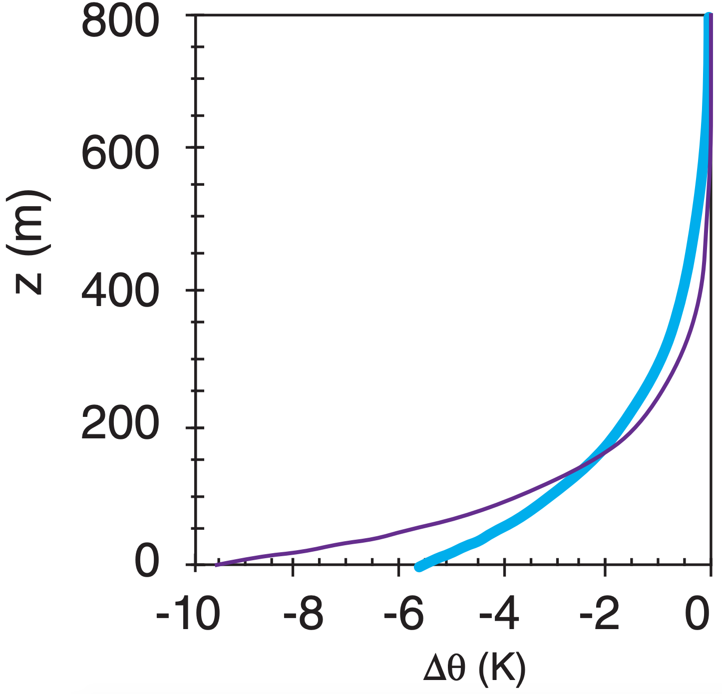
Check: Units OK, Physics OK. Graph OK.

Exposition: The windy case (thick cyan line) is not as cold near the ground, but the cooling extends over a greater depth than for the less-windy case (thin line).

18.4.4. Mixed-Layer (ML) Temperature

18.4.4.1. Evolution

The shape of the potential temperature profile in the mixed layer is simple. To good approximation it is uniform with height. Of more interest is the evolution of mixed-layer average θ and z_i with time.

Use the potential temperature profile at the end of the night (early morning) as the starting sounding for forecasting daytime temperature profiles. In real atmospheres, the sounding might not be a smooth exponential as idealized in the previous subsection. The method below works for arbitrary shapes of the initial potential temperature profile.

Figure 18.16 Evolution of the mixed layer with time, as cumulative heating increases the areas (hatched, then pink) under the curves.

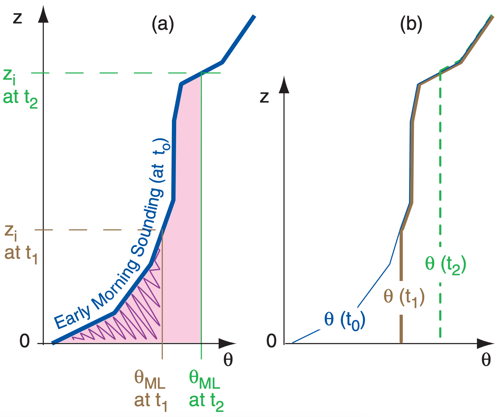
A graphical solution is easiest. First, plot the early-morning sounding of θ vs. z. Next, determine the cumulative daytime heating Q_Ak that occurs between sunrise and some time of interest t1, using eq. (18.2b). This heat warms the air in the ABL; thus the area under the sounding equals the accumulated heating (and also has units of K·m). Plot a vertical line of constant θ between the ground and the sounding, so that the area under the curve (hatched in Fig. 18.16a) equals the cumulative heating.

This vertical line gives the potential temperature of the mixed layer θ_ML(t₁). The height where this vertical line intersects the early-morning sounding defines the mixed-layer depth z_i (t₁). As cumulative heating increases with time during the day (Area₂ = total pink-shaded region at time t₂), the mixed layer becomes warmer and deeper (Fig. 18.16a). The resulting potential temperature profiles during the day are sketched in Fig. 18.16b. This method of finding mixed layer growth is called the encroachment method, or thermodynamic method, and explains roughly 90% of typical mixed-layer growth on sunny days with winds less than 10 m s^–1.

Sample Application

Given an early morning sounding with surface temperature 5°C and lapse rate ∆θ/∆z = 3 K km^–1. Find the mixed-layer potential temperature and depth at 10 AM, when the cumulative heating is 500 K·m.

Find the Answer

Given: θ_sfc = 5°C, ∆θ/∆z = 3 K km^–1, Q_Ak =0.50 K·km

Find: θ_ML = ? °C, z_i = ? km

Sketch:

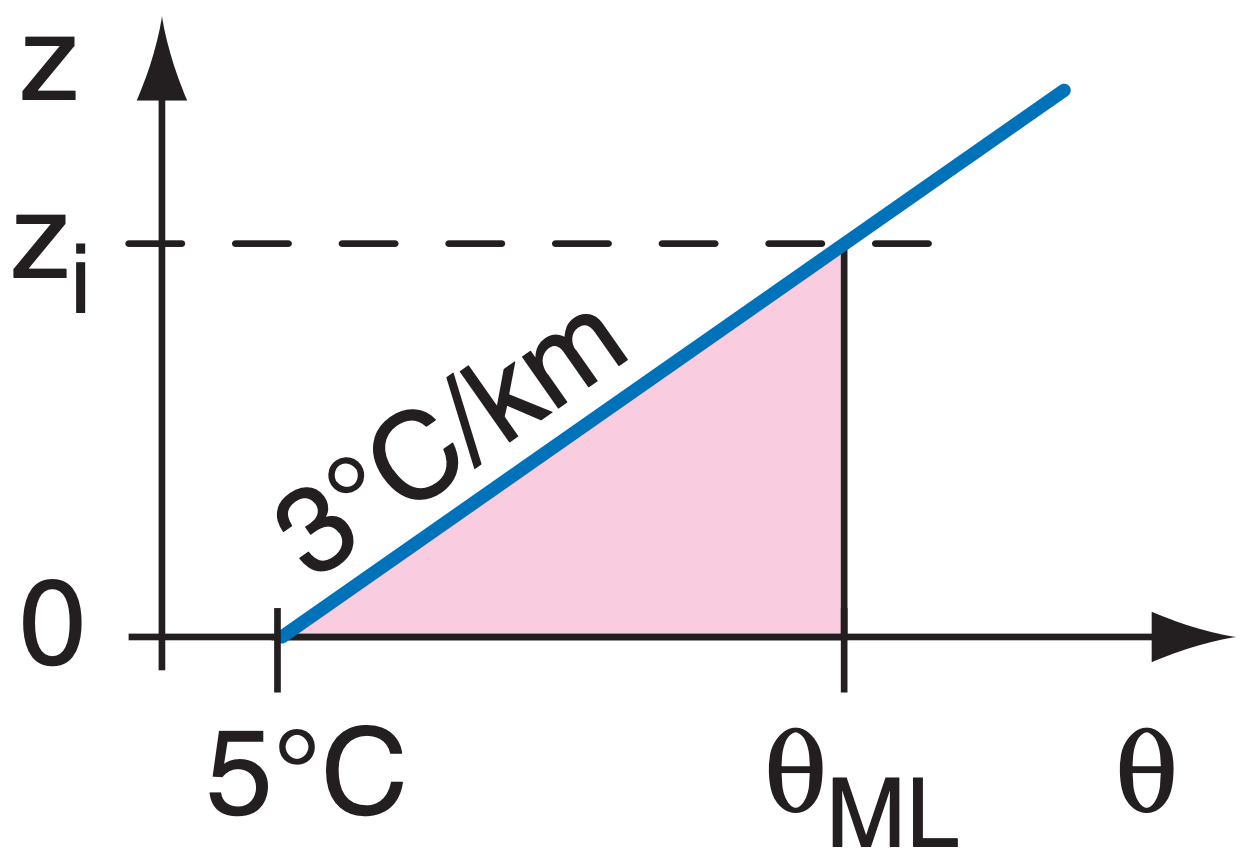
The area under this simple sounding is the area of a triangle: Area = 0.5·[base]·(height) , Area = 0.5·[(∆θ/∆z)·z_i ]·(z_i ) 0.50 K·km = 0.5·(3 K km^–1)·z_i²

Rearrange and solve for z_i :

z_i = 0.577 km

Next, use the sounding to find the θ_ML:

θ_ML = θ_sfc + (∆θ/∆z)·z_i

θ_ML = (5°C) + (3°C km^–1)·(0.577 km) = 6.73 °C

Check: Units OK. Physics OK. Sketch OK.

Exposition: Arbitrary soundings can be approximated by straight line segments. The area under such a sounding consists of the sum of areas within trapezoids under each line segment. Alternately, draw the early-morning sounding on graph paper, count the number of little grid boxes under the sounding, and multiply by the area of each box.

18.4.4.2. Entrainment

Figure 18.17 (a) Slab idealization of the mixed layer (solid line) approximates a more realistic potential temperature (θ) profile (dashed line). (b) Corresponding real and idealized heat flux (F_H) profiles.

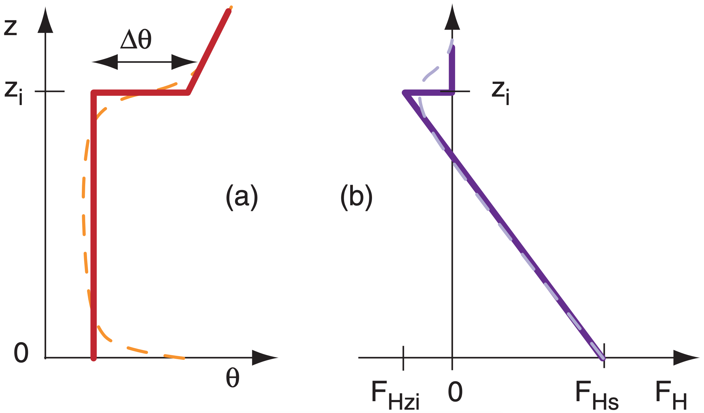
As was mentioned earlier, the turbulent mixed layer grows by entraining non-turbulent air from the free atmosphere. One can idealize the mixed layer as a slab model (Fig. 18.17a), with constant potential temperature in the mixed layer, and a jump of potential temperature (∆θ) at the EZ.

Entrained air from the free atmosphere has warmer potential temperature than air in the mixed layer. Because this warm air is entrained downward, it corresponds to a negative heat flux F_{H zi} at the top of the mixed layer. The heat-flux profile (Fig. 18.17b) is often linear with height, with the most negative value marking the top of the mixed layer.

The entrainment rate of free atmosphere air into the mixed layer is called the entrainment velocity, w_e, and can never be negative. The entrainment velocity is the volume of entrained air per unit horizontal area per unit time. In other words it is a volume flux, which has the same units as velocity.

The rate of growth of the mixed layer during fair weather is

\(\ \begin{align} \frac{\Delta z_{i}}{\Delta t}=w_{e}+w_{s}\tag{18.6}\end{align}\)

where w_s is the synoptic scale vertical velocity, and is negative for the subsidence that is typical during fair weather (recall Fig. 18.5).

The kinematic heat flux at the top of the mixed layer is

\(\ \begin{align} F_{H z i}=-w_{e} \cdot \Delta \theta\tag{18.7}\end{align}\)

where the sign and magnitude of the temperature jump is defined by ∆θ = θ(just above z_i ) – θ(just below z_i ). Greater entrainment across stronger temperature inversions causes greater heat-flux magnitude. Similar relationships describe entrainment fluxes of moisture, pollutants, and momentum as a function of the jumps in humidity, pollution concentration, and wind speed, respectively, at the ML top. As for temperature, the jump is defined as the value above z_i minus the value below z_i . Entrainment velocity has the same value for all variables.

During free convection (when winds are weak and thermal convection is strong), the entrained kinematic heat flux is approximately 20% of the surface heat flux:

\(\ \begin{align}F_{H z i} \cong-A \cdot F_{H s f c}\tag{18.8}\end{align}\)

where A = 0.2 is called the Ball ratio, and F_{H sfc} is the surface kinematic heat flux. This special ratio works only for heat, and does not apply to other variables. During windier conditions, A can be greater than 0.2. Eq. (18.8) was used in the Heat chapter to get the vertical heat-flux divergence (eq. 3.40 & 3.41), a term in the Eulerian heat budget.

Sample Application

The mixed layer depth increases at the rate of 300 m h^–1 in a region with weak subsidence of 2 mm s^–1. If the inversion strength is 0.5°C, estimate the surface kinematic heat flux.

Find the Answer

Given: w_s= –0.002 m s^–1, ∆z_i /∆t= 0.083 m s^–1, ∆θ = 0.5°C

Find: F_{H sfc} = ? °C·m s^–1

First, solve eq. (18.6) for entrainment velocity:

w_e = ∆z_i /∆t – w_s = [0.083 – (–0.002)] m s^–1 = 0.085 m s^–1

Next, use eq. (18.7):

F_Hzi = (–0.085 m s^–1)·(0.5°C) = –0.0425 °C·m s^–1

Finally, rearrange eq. (18.8):

F_{H sfc}= –F_Hzi/A= –(–0.0425 °C·m s^–1)/0.2 = 0.21°C·m s^–1

Check: Units OK. Magnitude and sign OK.

Exposition: Multiplying by ρ·C_P for the bottom of the atmosphere gives a dynamic heat flux of F_H = 259 W m^–2. This is roughly half of the value of max incoming solar radiation from Fig. 2.13 in the Solar & IR Radiation chapter.

Combining the two equations above gives an approximation for the entrainment velocity during free convection:

\(\ \begin{align}w_{e} \cong \frac{A \cdot F_{H s f c}}{\Delta \theta}\tag{18.9}\end{align}\)

Combining this with eq. (18.6) gives a mixed-layer growth equation called the flux-ratio method. From these equations, we see that stronger capping inversions cause slower growth rate of the mixed layer, while greater surface heat flux (e.g., sunny day over land) causes faster growth. The flux-ratio method and the thermodynamic method usually give equivalent results for mixed layer growth during free convection.

For stormy conditions near thunderstorms or fronts, the ABL top is roughly at the tropopause. Alternately, in the Atmos. Forces & Winds chapter (Mass Conservation section) are estimates of z_i for bad weather.

Sample Application

Find the entrainment velocity for a potential temperature jump of 2°C at the EZ, and a surface kinematic heat flux of 0.2 K·m s^–1.

Find the Answer

Given: F_{H sfc} = 0.2 K·m s^–1, ∆θ = 2 °C = 2 K

Find: w_e = ? m s^–1

Use eq. (18.9):

\(\ w_{e} \cong \frac{A \cdot F_{H s f c}}{\Delta \theta}=\frac{0.2 \cdot(0.2 \mathrm{K} \cdot \mathrm{m} / \mathrm{s})}{(2 \mathrm{K})}=\underline{\bf{0.02 \mathrm{m}} \mathrm{s}^{-1}} \)

Check: Units OK. Physics OK.

Exposition: While 2 cm s^–1 seems small, when applied over 12 h of daylight works out to z_i = 864 m, which is a reasonable mixed-layer depth.