15.4: Tornadoes

Tornadoes are violently rotating, small-diameter columns of air in contact with the ground. Diameters range from 10 to 1000 m, with an average of about 100 m. In the center of the tornado is very low pressure (order of 10 kPa lower than ambient).

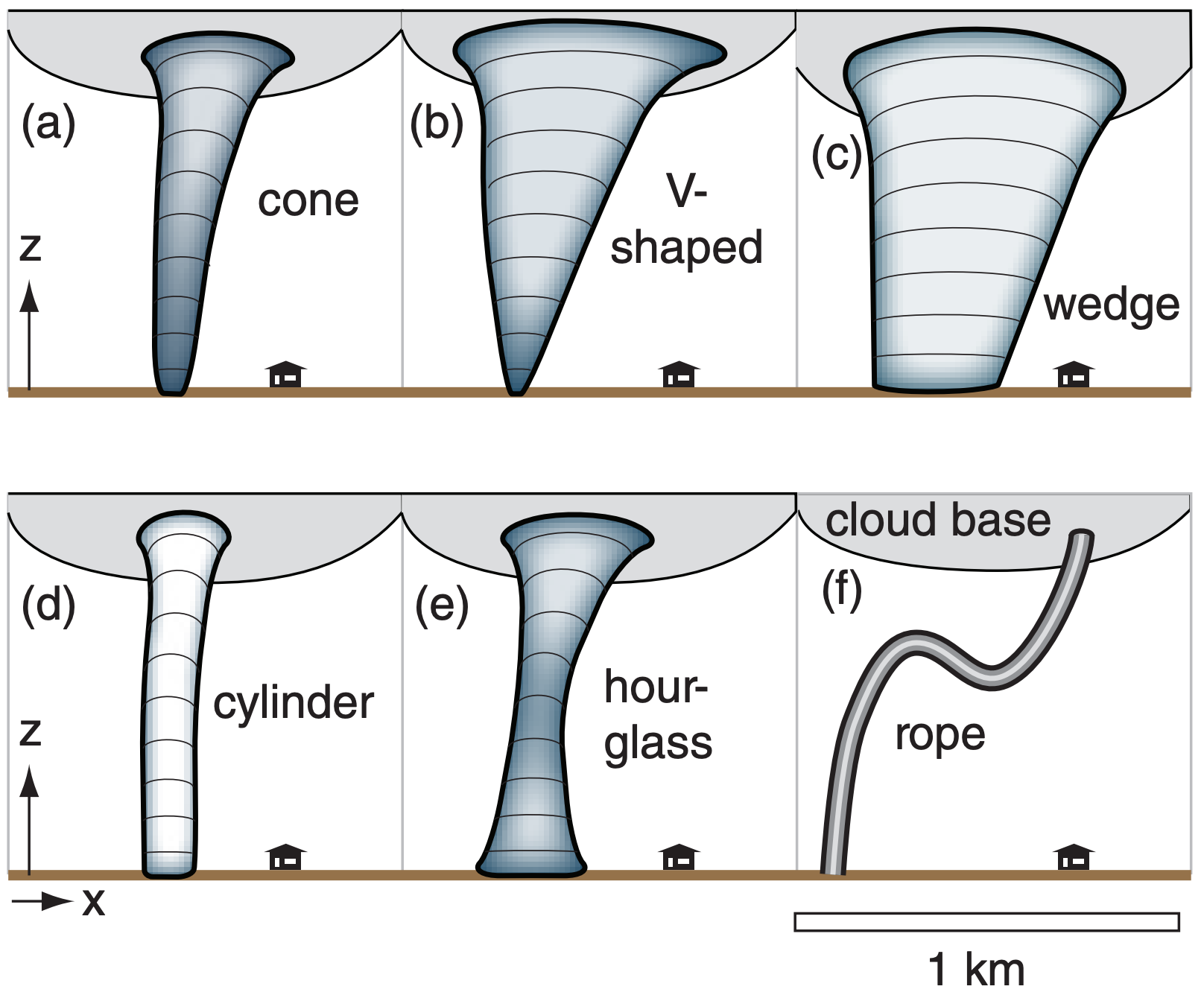
Tornadoes are usually formed by thunderstorms, but most thunderstorms do not spawn tornadoes. The strongest tornadoes come from supercell thunderstorms. Tornadoes have been observed with a wide variety of shapes (Fig. 15.32).

Figure 15.32 Illustration of some of the different tornado shapes observed.

15.4.1. Tangential Velocity & Tornado Intensity

Tangential velocities around tornadoes range from about 18 m s^–1 for weak tornadoes to greater than 140 m s^–1 for exceptionally strong ones. Tornado rotation is often strongest just above the ground (15 to 150 m AGL), where upward vertical velocities of 25 to 60 m s^–1 have been observed in the outer wall of the tornado. This combination of updraft and rotation can rip trees, animals and buildings from the ground and destroy them. It can also loft trucks, cars, and other large and small objects, which can fall outside the tornado path causing more damage.

Often a two-region model is used to approximate tangential velocity M_tan in a tornado, with an internal core region of radius R_o surrounded by an external region. R_o corresponds to the location of fastest tangential velocity M_{tan max} (Fig. 15.33), which is sometimes assumed to coincide with the outside edge of the visible funnel. Air in the core of the tornado rotates as a solid-body, while air outside the core is irrotational (has no relative vorticity as it moves around the tornado axis), and conserves angular momentum as it is drawn into the tornado. This model is called a Rankine combined vortex (RCV).

Figure 15.33 A Rankine-combined-vortex (RCV) model for tornado tangential velocity and pressure. The pressure deficit is plotted with reversed ordinate, indicating lower pressure in the tornado core.

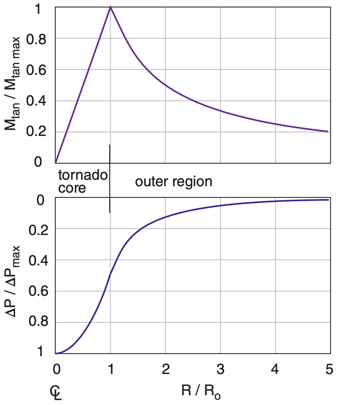
The pressure deficit is ∆P = P∞ – P , where P is the pressure at any radius R from the tornado axis, and P∞ is ambient pressure far away from the tornado (for P∞ ≥ P ). At R_o, the inner (core) and outer tangential wind speeds match, and the inner and outer pressure deficits match. Thus:

Core Region (R < R_o):

\(\ \begin{align} \frac{M_{\tan }}{M_{\tan \max }}=\frac{R}{R_{o}}\tag{15.40}\end{align}\)

\(\ \begin{align} \frac{\Delta P}{\Delta P_{\max }}=1-\frac{1}{2}\left(\frac{R}{R_{0}}\right)^{2}\tag{15.41}\end{align}\)

Outer Region (R > R_o):

\(\ \begin{align} \frac{M_{\tan }}{M_{\tan \max }}=\frac{R_{0}}{R}\tag{15.42}\end{align}\)

\(\ \begin{align} \frac{\Delta P}{\Delta P_{\max }}=\frac{1}{2}\left(\frac{R_{o}}{R}\right)^{2}\tag{15.43}\end{align}\)

These equations are plotted in Fig. 15.33, and represent the wind relative to that in the center of the tornado.

Max tangential velocity (at R = R_o) and max core pressure deficit (∆P_max , at R = 0) are related by

\(\ \begin{align} \Delta P_{\max }=\rho \cdot\left(M_{\tan \max }\right)^{2}\tag{15.44}\end{align}\)

where ρ is air density. This equation was derived from the Bernoulli equation. M_{tan max} can also be described as a cyclostrophic wind as explained in the Forces & Winds chapter (namely, it is a balance between centrifugal and pressure-gradient forces). Forecasting these maximum values is difficult.

Near the Earth’s surface, frictional drag near the ground slows the air below the cyclostrophic speed. Thus there is insufficient centrifugal force to balance pressure-gradient force, which allows air to be sucked into the bottom of the tornado. Further away from the ground, the balance of forces causes zero net radial flow across the tornado walls; hence, the tornado behaves similar to a vacuum-cleaner hose.

Figure 15.34 Illustration of sum of relative rotational (M_tan) wind and tornado translation (M_tr) to yield total winds (M_total) measured at the ground. Tornado intensity is classified based on the maximum wind speed (M_max) anywhere in the tornado.

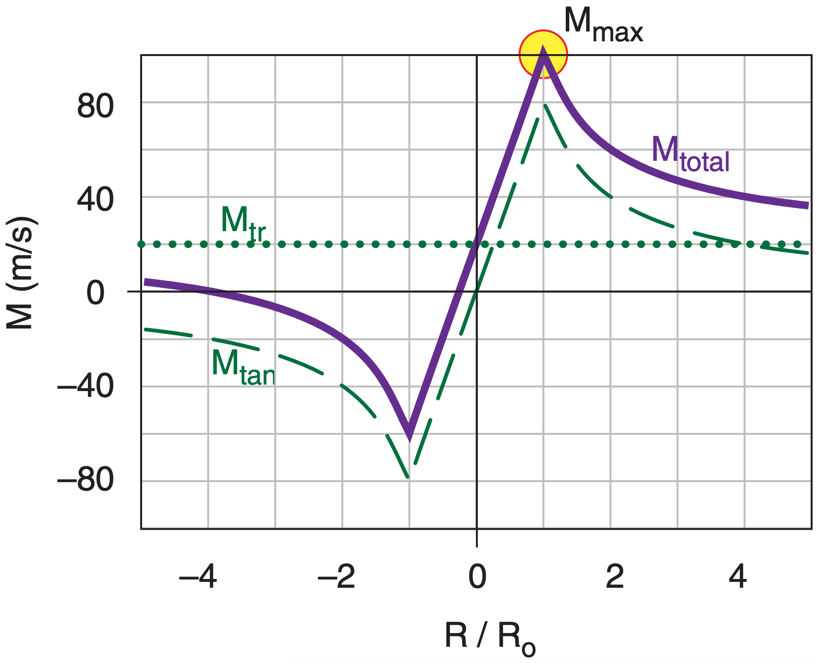
The previous 5 equations gave tangential wind speed relative to the center of the tornado. But the tornado also moves horizontally (translates) with its parent thunderstorm. The total wind M_total at any point near the tornado is the vector sum of the rotational wind M_tan plus the translational wind M_tr (Fig. 15.34). The max wind speed M_max associated with the tornado is

\(\ \begin{align} \left|M_{\max }\right|=\left|M_{\tan \max }\right|+\left|M_{t r}\right|\tag{15.45}\end{align}\)

and is found on the right side of the storm (relative to its translation direction) for cyclonically (counterclockwise, in the Northern Hemisphere) rotating tornadoes.

Most tornadoes rotate cyclonically. Less than 2% of tornadoes rotate the opposite direction (anticyclonically). This low percentage is due to two factors: (1) Coriolis force favors mesocyclones that rotate cyclonically, and (2) friction at the ground causes a turning of the wind with increasing height (Fig. 15.42, presented in a later section), which favors right-moving supercells in the Northern Hemisphere with cyclonically rotating tornadoes.

Sample Application

If the max pressure deficit in the center of a 20 m radius tornado is 10 kPa, find the max tangential wind speed, and the wind and pressure deficit at R = 50 m.

Find the Answer

Given: R_o = 20 m, ∆P_max = 10 kPa, R = 50 m

Find: M_{tan max} = ? m s^–1.

Also M_tan = ? m s^–1 and ∆P = ? kPa at R = 50 m. Assume: ρ = 1 kg m^–3.

Use eq. (15.44):

M_{tan max} = [∆P_max/ ρ] ^1/2 = [(10,000 Pa) / (1 kg m^–3)]^1/2 = 100 m s^–1

Because R > R_o, use outer-region eqs. (15.42 & 15.43):

M_tan = (100 m s^–1) · [(20 m)/(50 m)] = 40 m s^–1

∆P = 0.5·(10 kPa) · [(20 m)/(50 m)]² = 0.8 kPa.

Check: Physics OK. Units OK. Agrees with Fig. 15.33.

Exposition: 10 kPa is quite a large pressure deficit in the core — roughly 10% of sea-level pressure. However, most tornadoes are not this violent. Typical tangential winds of 60 m s^–1 or less would correspond to core pressure deficits of 3.6 kPa or less.

One tornado damage scale was devised by the Tornado and Storm Research Organization in Europe, and is called the TORRO scale (T). Another scale was developed for North America by Ted Fujita, and is called the Fujita scale (F).

In 2007 the Fujita scale was revised into an Enhanced Fujita (EF) scale (Table 15-3), based on better measurements of the relationship between winds and damage for 28 different types of structures. It is important to note that the EF intensity determination for any tornado is based on a damage survey AFTER the tornado has happened.

For example, consider modern, well-built singlefamily homes and duplexes, typically built with wood or steel studs, with plywood roof and outside walls, all covered with usual types of roofing, sidings, or brick. For this structure, use the following damage descriptions to estimate the EF value:

• If near the threshold of visible damage, then EF0 or less.
• If loss of gutters, or awnings, or vinyl or metal siding, or less than 20% of roof covering material, then EF0 - EF1.
• If broken glass in doors and windows, or roof lifted up, or more than 20% of roof covering missing, or chimney collapse, or garage doors collapse inward, or failure of porch or carport, then EF0 - EF2.
• If entire house shifts off foundation, or large sections of roof structure removed (but most walls remain standing), then EF1 - EF3.
• If exterior walls collapse, then EF2 - EF3.
• If most walls collapse, except small interior rooms, then EF2 - EF4.
• If all walls collapse, then EF3 - EF4.
• If total destruction & floor slabs swept clean, then EF4 - EF5.

Similar damage descriptions for the other 27 types of structures (including trees) are available from the USA Storm Prediction Center.

For any EF value (such as EF = 4), the lower threshold of maximum tangential 3-second-gust wind speed M_max is approximately:

\(\ \begin{align} M_{\max }=M_{o}+a \cdot(\mathrm{EF})^ {1.2}\tag{15.46}\end{align}\)

where M_o = 29.1 m s^–1 and a = 8.75 m s^–1.

The “derived” gust thresholds listed in Table 15-3 are often converted to speed units familiar to the public and then rounded to pleasing integers of nearly the correct value. Such a result is known as an Operational Scale (see Table 15-3).

Table 15-3. Enhanced Fujita scale for tornado-damage intensity. (Derived-scale speeds from NOAA Storm Prediction Center.)
Scale	Derived Max Tangential 3 s Gust Speed (m/s)	Operational Scales		Damage Classification Description (from the old Fujita F scale)	Relative Frequency
		EF Scale (stat. miles/h)	Old F Scale (km/h)		USA	Canada
EF0	29.1 – 38.3	65 – 85	64 – 116	Light damage; some damage to chimneys, TV antennas; breaks twigs off trees; pushes over shallow-rooted trees.	29%	45%
EF1	38.4 – 49.1	86 – 110	117 – 180	Moderate damage; peels surface off roofs; windows broken; light trailer homes pushed or turned over; some trees uprooted or snapped; moving cars pushed off road.	40%	29%
EF2	49.2 – 61.6	111 – 135	181 – 252	Considerable damage; roofs torn off wood-frame houses leaving strong upright walls; weak buildings in rural areas demolished; mobile homes destroyed; large trees snapped or uprooted; railroad boxcars pushed over; light object missiles generated; cars blown off roads.	24%	21%
EF3	61.7 – 75.0	136 – 165	253 – 330	Severe damage; roofs and some walls torn off wood-frame houses; some rural buildings completely destroyed; trains overturned; steel-framed hangars or warehouse-type structures torn; cars lifted off of the ground; most trees in a forest uprooted or snapped and leveled.	6%	4%
EF4	75.1 – 89.3	166 – 200	331 – 417	Devastating damage; whole wood-frame houses leveled leaving piles of debris; steel structures badly damaged; trees debarked by small flying debris; cars and trains thrown or rolled considerable distances; large wind-blown missiles generated.	2%	1%
EF5	≥ 89.4	> 200	418 – 509	Incredible damage; whole wood-frame houses tossed off foundation and blown downwind; steel-reinforced concrete structures badly damaged; automobile-sized missiles generated; incredible phenomena can occur.	< 1%	0.1%

Tornado intensity varies during the life-cycle of the tornado, so different levels of destruction are usually found along the damage path for any one tornado. Tornadoes of strength EF2 or greater are labeled significant tornadoes.

The TORRO scale (Table 15-4) is defined by maximum wind speed M_max, but in practice is estimated by damage surveys. The lower threshold of windspeed for any T value (e.g., T7) is defined approximately by:

\(\ \begin{align} M_{\max } \approx a \cdot(\mathbf{T}+4)^{1.5}\tag{15.47}\end{align}\)

where a = 2.365 m s^–1 and T is the TORRO tornado intensity value. A weak tornado would be classified as T0, while an extremely strong one would be T10 or higher.

Any tornado-damage scale is difficult to use and interpret, because there are no actual wind measurements for most events. However, the accumulation of tornado-damage-scale estimates provides valuable statistics over the long term, as individual errors are averaged out.

Sample Application

Find Enhanced Fujita & TORRO intensities for M_max = 100 m s^–1.

Find the Answer

Given: M_max= 100 m s^–1.

Find: EF and T intensities

Use Tables 15-3 and 15-4: ≈ EF5 , T8 .

Exposition: This is a violent, very destructive, significant tornado.

Table 15-4. TORRO tornado scale. (from www.torro.org.uk/site/tscale.php)
Scale	Max. Speed (m s^–1)	Tornado Intensity & Damage Description (Abridged from the Torro web site) [UK “articulated lorry” ≈ USA “semi-trailer truck” or “semi”]
T0	17 – 24	Light. Loose light litter raised from ground in spirals; tents, marquees disturbed; exposed tiles & slates on roofs dislodged; twigs snapped; visible damage path through crops.
T1	25 – 32	Mild. Deck chairs, small plants, heavy litter airborne; dislodging of roof tiles, slates, and chimney pots; wooden fences flattened; slight damage to hedges and trees.
T2	33 – 41	Moderate. Heavy mobile homes displaced; semis blown over; garden sheds destroyed; garage roofs torn away; damage to tile and slate roofs and chimney pots; large tree branches snapped; windows broken.
T3	42 – 51	Strong. Mobile homes overturned & badly damaged; light semis destroyed; garages and weak outbuildings destroyed; much of the roofing material removed; some larger trees uprooted or snapped.
T4	52 – 61	Severe. Cars lifted; mobile homes airborne & destroyed; sheds airborne for considerable distances; entire roofs removed; gable ends torn away; numerous trees uprooted or snapped.
T5	62 – 72	Intense. Heavy motor vehicles lifted (e.g., 4 tonne trucks); more house damage than T4; weak buildings completely collapsed; utility poles snapped.
T6	73 – 83	Moderately Devastating. Strongly built houses lose entire roofs and perhaps a wall; weaker built structures collapse completely; electric-power transmission pylons destroyed; objects embedded in walls.
T7	84 – 95	Strongly Devastating. Wooden-frame houses wholly demolished; some walls of stone or brick houses collapsed; steel-framed warehouse constructions buckled slightly; locomotives tipped over; noticeable debarking of trees by flying debris.
T8	96 – 107	Severely Devastating. Cars hurled great distances; wooden-framed houses destroyed and contents dispersed over large distances; stone and brick houses irreparably damaged; steel-framed buildings buckled.
T9	108 – 120	Intensely Devastating. Many steel-framed buildings badly demolished; locomotives or trains hurled some distances; complete debarking of standing tree trunks.
T10	121 – 134	Super. Entire frame houses lifted from foundations, carried some distances & destroyed; severe damage to steel-reinforced concrete buildings; damage track left with nothing standing above ground.

15.4.2. Appearance

Two phenomena can make tornadoes visible: water droplets and debris (Fig. 15.35). Sometimes these processes make only the bottom or top part of the tornado visible; rarely, the whole tornado is invisible. Regardless of whether you can see the tornado, if the structure consists of a violently rotating column of air, then it is classified as a tornado.

Figure 15.35 Condensation funnel and debris cloud.

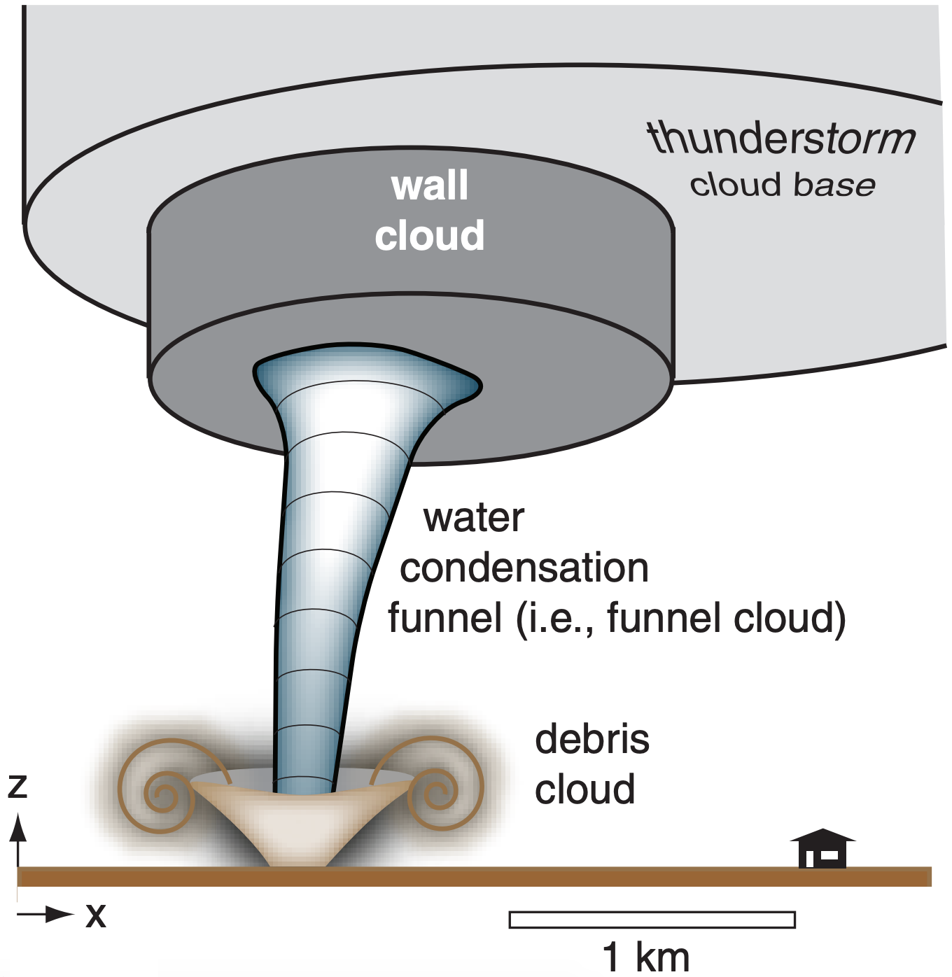
Debris can be formed as the tornado destroys things on the Earth’s surface. The resulting smaller fragments (dirt, leaves, grass, pieces of wood, bugs, building materials and papers from houses and barns) are drawn into the tornado wall and upward, creating a visible debris cloud. (Larger items such as whole cars can be lifted by the more intense tornadoes and tossed outward, some as much as 30 m.) If tornadoes move over dry ground, the debris cloud can include dust and sand. Debris clouds form at the ground, and can extend to various heights for different tornadoes, including some that extend up to wall-cloud base.

The water-condensation funnel is caused by low pressure inside the tornado, which allows air to expand as it is sucked horizontally toward the core. As the air expands it cools, and can reach saturation if the pressure is low enough and the initial humidity of the air is great enough. The resulting cloud of water droplets is called a funnel cloud, and usually extends downward from the thunderstorm cloud base. Sometimes this condensation funnel cloud can reach all the way to the ground. Most strong tornadoes have both a condensation funnel and a debris cloud (Fig. 15.35).

Because the tornado condensation funnel is formed by a process similar to the lifting condensation level (LCL) for normal convective cloud base, you can use the same LCL equation (see the Water Vapor chapter) to estimate the pressure P_cf at the outside of the tornado condensation funnel, knowing the ambient air temperature T and dew point Td at ambient near-surface pressure P. Namely, P_cf = P_LCL.

\(\ \begin{align} P_{c f}=P \cdot\left[1-b \cdot\left(\frac{T-T_{d}}{T}\right)\right]^{C_{p} / \Re}\tag{15.48}\end{align}\)

where C_p/ℜ = 3.5 and b = 1.225 , both dimensionless, T and T_d in the numerator must be in the same units, and where T in the denominator must be in Kelvin.

Figure 15.36 Relationship between lifting-condensation-level pressure (P_LCL), cloud base, and pressure at the condensation funnel (P_cf). Horizontal pressure gradient at point “A” is 4 times that at “B”.

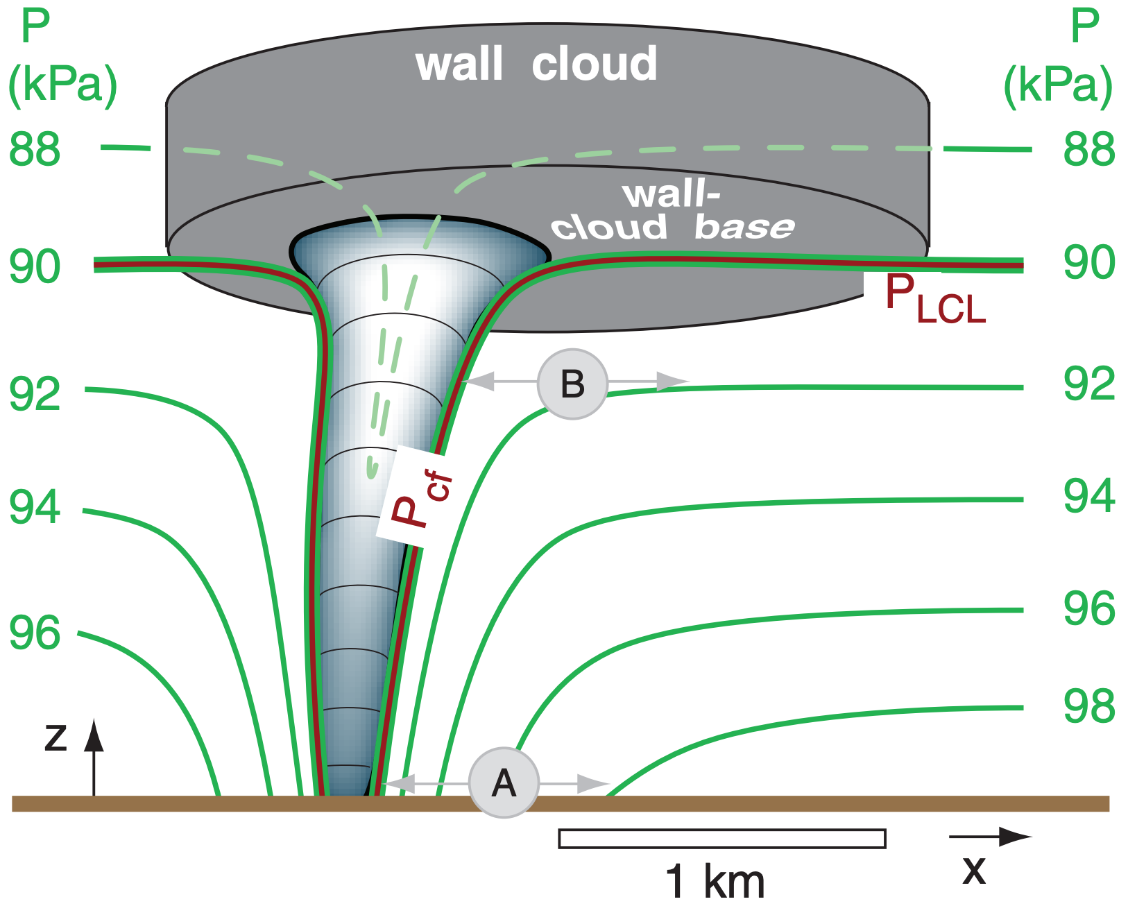
Assuming both the condensation funnel and cloud base indicate the same pressure, the isobars must curve downward near the tornado (Fig. 15.36). Thus, the greatest horizontal pressure gradient associated with the tornado is near the ground (near “A” in Fig. 15.36). Drag at the ground slows the wind a bit there, which is why the fastest tangential winds in a tornado are found 15 to 150 m above ground.

Sample Application

Under a tornadic thunderstorm, the temperature is 30°C and dew point is 23°C near the ground where pressure is 100 kPa. Find the near-surface pressure at the outside edge of the visible condensation funnel.

Find the Answer

Given: T = 30°C = 303K , T_d = 23°C , P = 100 kPa

Find: P_cf = ? kPa

Use eq. (15.48): P_cf = (100kPa)·[ 1 – 1.225·(30–23)/303]^3.5 = 90.4 kPa at the tornado funnel-cloud edge.

Check: Units OK. Physics OK.

Exposition: The tornado core pressure can be even lower than at the edge of the condensation funnel.

15.4.3. Types of Tornadoes & Other Vortices

Figure 15.37 Illustration of tornado and vortex types.

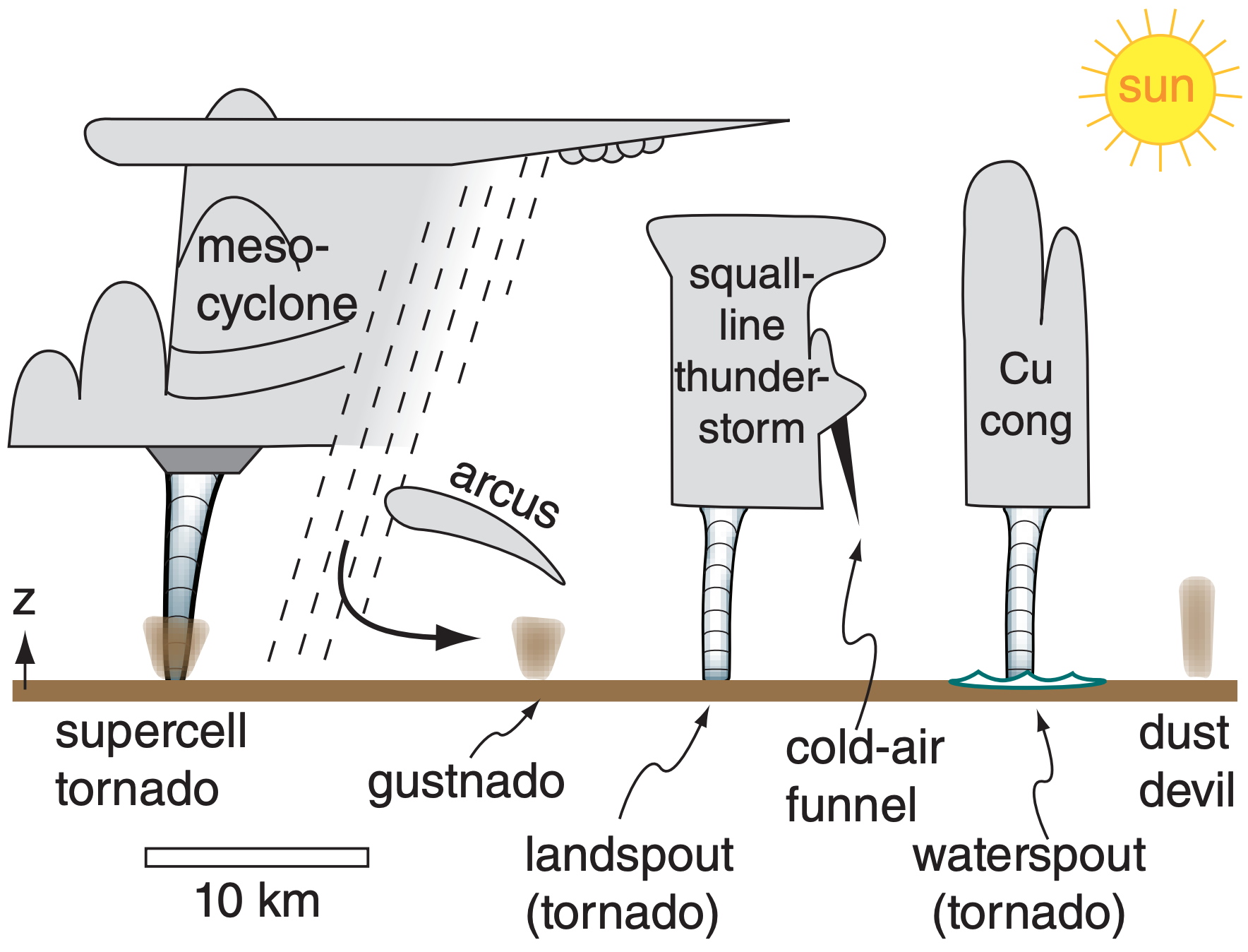
We will compare six types of vortices (Fig 15.37):

• supercell tornadoes
• landspout tornadoes
• waterspouts
• cold-air funnels
• gustnadoes
• dust devils, steam devils, firewhirls

Recall from the Thunderstorm chapter that a mesocyclone is where the whole thunderstorm updraft (order of 10 to 15 km diameter) is slowly rotating (often too slowly to see by eye). This rotation can last for 1 h or more, and is one of the characteristics of a supercell thunderstorm. Only a small percentage of thunderstorms are supercells with mesocyclones, but it is from these supercells that the strongest tornadoes can form. Tornadoes rotate faster and have smaller diameter (~100 m) than mesocyclones.

Supercell tornadoes form under (and are attached to) the main updraft of supercell thunderstorms (Figs. 15.32a-c, 15.35, & 15.37) or under a cumulus congestus that is merging into the main supercell updraft from the flanking line. It can be the most violent tornado type — up through EF5 intensity. They move horizontally (i.e., translate) at nearly the same speed as the parent thunderstorm (on the order of 5 to 40 m s^–1). These tornadoes will be discussed in more detail in the next subsections.

Landspouts are weaker tornadoes (EF0 - EF2, approximately) not usually associated with supercell thunderstorms. They are often cylindrical, and look like hollow soda straws (Fig. 15.32d). These shortlived tornadoes form along strong cold fronts. Horizontal wind shear across the frontal zone provides the rotation, and vertical stretching of the air by updrafts in the squall-line thunderstorms along the front can intensify the rotation (Fig. 15.37).

Waterspouts (Fig. 15.37) are tornadoes that usually look like landspouts (hollow, narrow, 3 to 100 m diameter cylinders), but form over water surfaces (oceans, lakes, wide rivers, bays, etc.). They are often observed in subtropical regions (e.g., in the waters around Florida), and can form under (and are attached to) cumulus congestus clouds and small thunderstorms. They are often short lived (usually 5 to 10 min) and weak (EF0 - EF1). The waterspout life cycle is visible by eye via changes in color and waves on the water surface: (1) dark spot, (2) spiral pattern, (3) spray-ring, (4) mature spray vortex, and (5) decay. Waterspouts have also been observed to the lee of mountainous islands such as Vancouver Island, Canada, where the initial rotation is caused by wake vortices as the wind swirls around the sides of mountains.

Unfortunately, whenever any type of tornado moves over the water, it is also called a waterspout.

Thus, supercell tornadoes (EF3 - EF5) would be called waterspouts if they moved over water. So use caution when you hear waterspouts reported in a weather warning, because without other information, you won’t know if it is a weak classical waterspout or a strong tornado.

Cold-air funnels are short vortices attached to shallow thunderstorms with high cloud bases, or sometimes coming from the sides of updraft towers (Fig. 15.37). They are very short lived (1 - 3 minutes), weak, and usually don’t reach the ground. Hence, they usually cause no damage on the ground (although light aircraft should avoid them). Cold-air funnels form in synoptic cold-core low-pressure systems with a deep layer of unstable air.

Gustnadoes are shallow (order of 100 m tall) debris vortices touching the ground (Fig. 15.37). They form along the gust-front from thunderstorms, where there is shear between the outflow air and the ambient air. Gustnadoes are very weak (EF0 or weaker) and very short lived (a few minutes). The arc clouds along the gust front are not usually convective, so there is little or no updraft to stretch the air vertically, and hence no mechanism for accelerating the vorticity. There might also be rotation or a very small condensation funnel visible in the overlying arc clouds. Gustnadoes translate with the speed of advance of the gust front.

Dust devils are not tornadoes, and are not associated with thunderstorms. They are fair-weather phenomena, and can form in the clear-air thermals of warm air rising from a heated surface (Fig. 15.37). They are weak (less than EF0) debris vortices, where the debris can be dust, sand, leaves, volcanic ash, grass, litter, etc. Normally they form during daytime in high-pressure regions, where the sun heats the ground, and are observed over the desert or other arid locations. They translate very slowly or not at all, depending on the ambient wind speed.

When formed by arctic-air advection over an unfrozen lake in winter, the resulting steam-devils can happen day or night. Smoky air heated by forest fires can create firewhirls. Dust devils, steam devils, firewhirls and gustnadoes look very similar.

15.4.4. Evolution as Observed by Eye

From the ground, the first evidence of an incipient supercell tornado is a dust swirl near the ground, and sometimes a rotating wall cloud protruding under the thunderstorm cloud base (Fig. 15.38). Stage 2 is the developing stage, when a condensation funnel cloud begins to extend downward from the bottom of the wall cloud or thunderstorm base, and the debris cloud becomes larger with well-defined rotation.

Figure 15.38 Stages in a supercell-tornado life cycle. Caution: the EF intensity of some tornadoes can fluctuate while the tornado is in its mature stage (stage 3).

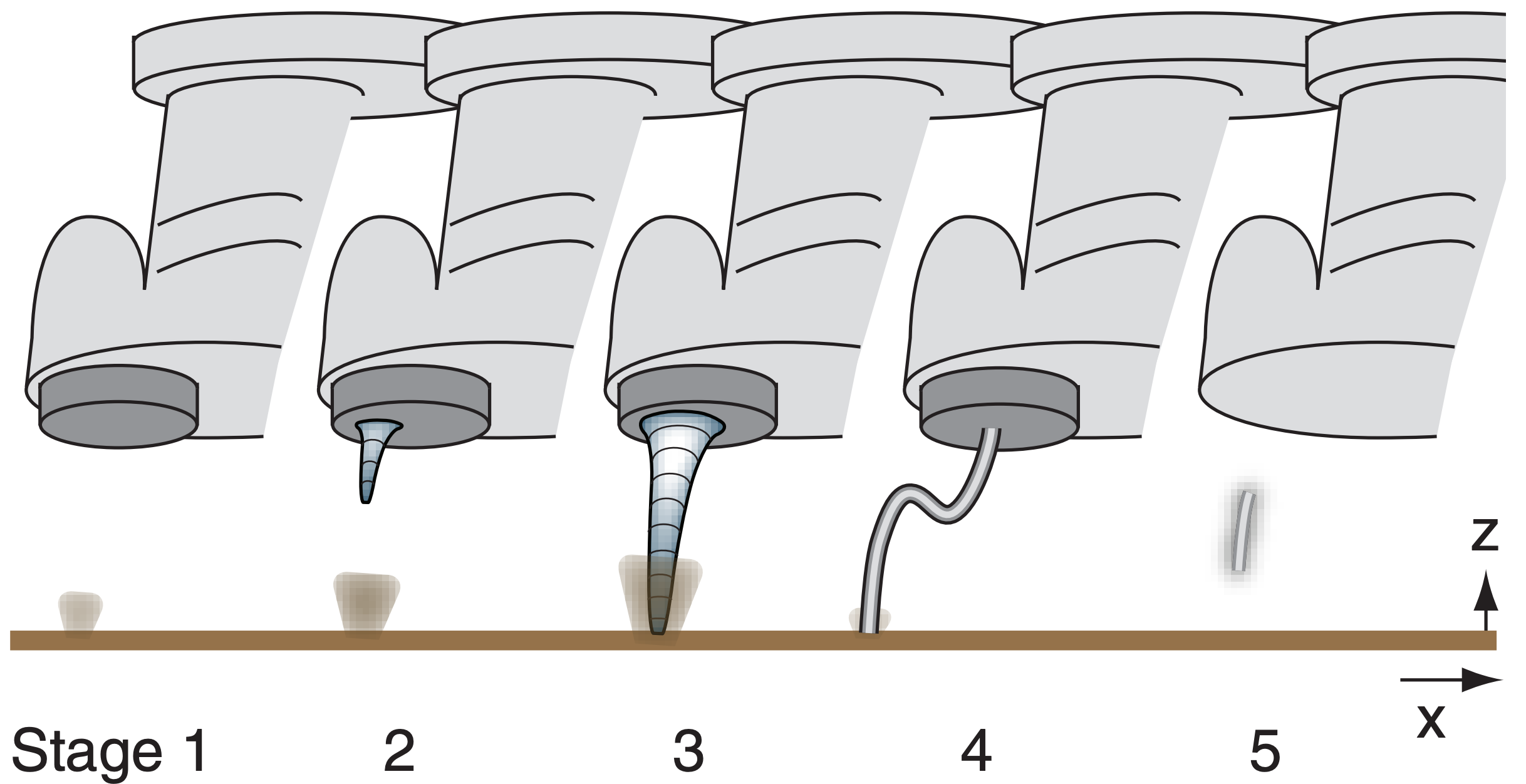
Stage 3 is the mature stage, when there is a visible column of rotating droplets and/or debris extending all the way from the cloud to the ground. This is the stage when tornadoes are most destructive. During stage 4 the visible tornado weakens, and often has a slender rope-like shape (also in Fig. 15.32f). As it dissipates in stage 5, the condensation funnel disappears up into the cloud base and the debris cloud at the surface weakens and disperses in the ambient wind. Meanwhile, a cautious storm chaser will also look to the east or southeast under the same thunderstorm cloud base, because sometimes new tornadoes form there.

15.4.5. Tornado Outbreaks

A tornado outbreak is when a single synoptic-scale system (e.g., cold front) spawns ten or more tornadoes during one to seven days (meteorologists are still debating a more precise definition). Tornado outbreaks have been observed every decade in North America for the past couple hundred years of recorded meteorological history. Outbreaks often occur one or more times each year.

The following list highlights a small portion of the outbreaks in North America:

• 25 May - 1 June 1917: 63 tornadoes in Illinois killed 383 people.
• 18 March 1925 (tri-state) Tornado: Deadliest tornado(es) in USA, killing 695 people on a 350 km track through Missouri, Illinois & Indiana.
• 1 - 9 May 1930: 67 tornadoes in Texas killed 110.
• 5 - 6 April 1936: 17 tornadoes in Tupelo, Mississippi, and Gainesville, Georgia, killed 454.
• 7 - 11 April 1965 (Palm Sunday): 51 F2 - F5 tornadoes, killed 256.
• 3 - 4 April 1974: 148 tornadoes, killed 306 people in Midwest USA, and 9 in Canada.
• 31 May 1985: 41 tornadoes near the USA-Canada border killed 76 in USA and 12 in Canada.
• 3 - 11 May 2003: 401 tornadoes in tornado alley (central USA) killed 48.
• September 2004 in Hurricanes Francis & Ivan: 220 tornadoes.
• 22 - 25 May 2008: 234 tornadoes in central USA killed 10.
• 25 - 28 April 2011: 362 tornadoes in E. USA, killed 324, causing about $10 billion in damage.
• 21 - 26 May 2011: 241 tornadoes in midwest USA killed 178.

Outbreaks are often caused by a line or cluster of supercell thunderstorms. Picture a north-south line of storms, with each thunderstorm in the line marching toward the northeast together like troops on parade (Fig. 15.39). Each tornadic supercell in this line might create a sequence of multiple tornadoes (called a tornado family), with very brief gaps between when old tornadoes decay and new ones form. The aftermath includes parallel tornado damage paths like a wide (hundreds of km) multilane highway oriented usually from southwest toward northeast in North America.

A SCIENTIFIC PERSPECTIVE • Be Safe (part 4)

More chase guidelines from Charles Doswell III.

The #3 Threat: The Storm

1. Avoid driving through the heaviest precipitation part of the storm (known as “core punching”).
2. Avoid driving under, or close to, rotating wall clouds.
3. Don’t put yourself in the path of a tornado or a rotating wall cloud.
4. You must also be aware of what is happening around you, as thunderstorms and tornadoes develop quickly. You can easily find yourself in the path of a new thunderstorm while you are focused on watching an older storm. Don’t let this happen — be vigilant.
5. For new storm chasers, find an experienced chaser to be your mentor. (Work out such an arrangement ahead of time; don’t just follow an experienced chaser uninvited.)
6. Keep your engine running when you park to view the storm.
7. Even with no tornado, straight-line winds can move hail or debris (sheet metal, fence posts, etc.) fast enough to kill or injure you, and break car windows. Move away from such regions.
8. Avoid areas of rotating curtains of rain, as these might indicate that you are in the dangerous center of a mesocyclone (called the “bear’s cage”).
9. Don’t be foolhardy. Don’t be afraid to back off if your safety factor decreases.
10. Never drive into rising waters. Some thunderstorms such as HP supercell storms can cause flash floods.
11. Always have a clear idea of the structure, evolution, and movement of the storm you are viewing, so as to anticipate safe courses of action.

A SCIENTIFIC PERSPECTIVE • Be Safe (part 5)

More chase guidelines from Charles Doswell III.

The #3 Threat: The Storm (continuation)

12. Plan escape routes in advance.
13. Although vehicles offer safety from lightning, they are death traps in tornadoes. If you can’t drive away from the tornado, then abandon your vehicle and get into a ditch or culvert, or some other place below the line-of-fire of flying debris.
14. In open rural areas with good roads, you can often drive away from the tornado’s path.
15. Don’t park under bridge overpasses, because winds accelerate there & cause increased damage.
16. Avoid chasing at night. Keep in mind the following challenges:
    1. Storm movement as broadcast on radio or TV cannot be trusted. Often, the media reports the heavy precipitation areas, not the action (dangerous) areas of the mesocyclone and tornado.
    2. Storm info provided via various wireless data and internet services can be several minutes old or older.
    3. It is difficult to see tornadoes at night. Flashes of light from lightning & exploding electrical transformers (known as “power flashes”) are often inadequate to see the tornado. Also, not all power flashes are caused by tornadoes.
    4. If you find yourself in a region of strong inflow winds that are backing (changing direction counterclockwise), then you might be in the path of a tornado.
    5. Flooded roads are hard to see at night, and can cut off your escape routes. Your vehicle could hydroplane due to water on the road, causing you to lose control.
    6. Even after you stop chasing storms for the day, dangerous weather can harm you on your drive home or in a motel.

On his web site, Doswell offers many more tips and recommendations for responsible storm chasing.

15.4.6. Storm-relative Winds

Because tornadoes translate with their parent thunderstorms, the winds that influence supercell and tornado rotation are the environmental wind vectors relative to a coordinate system that moves with the thunderstorm. Such winds are called storm-relative (SR) winds.

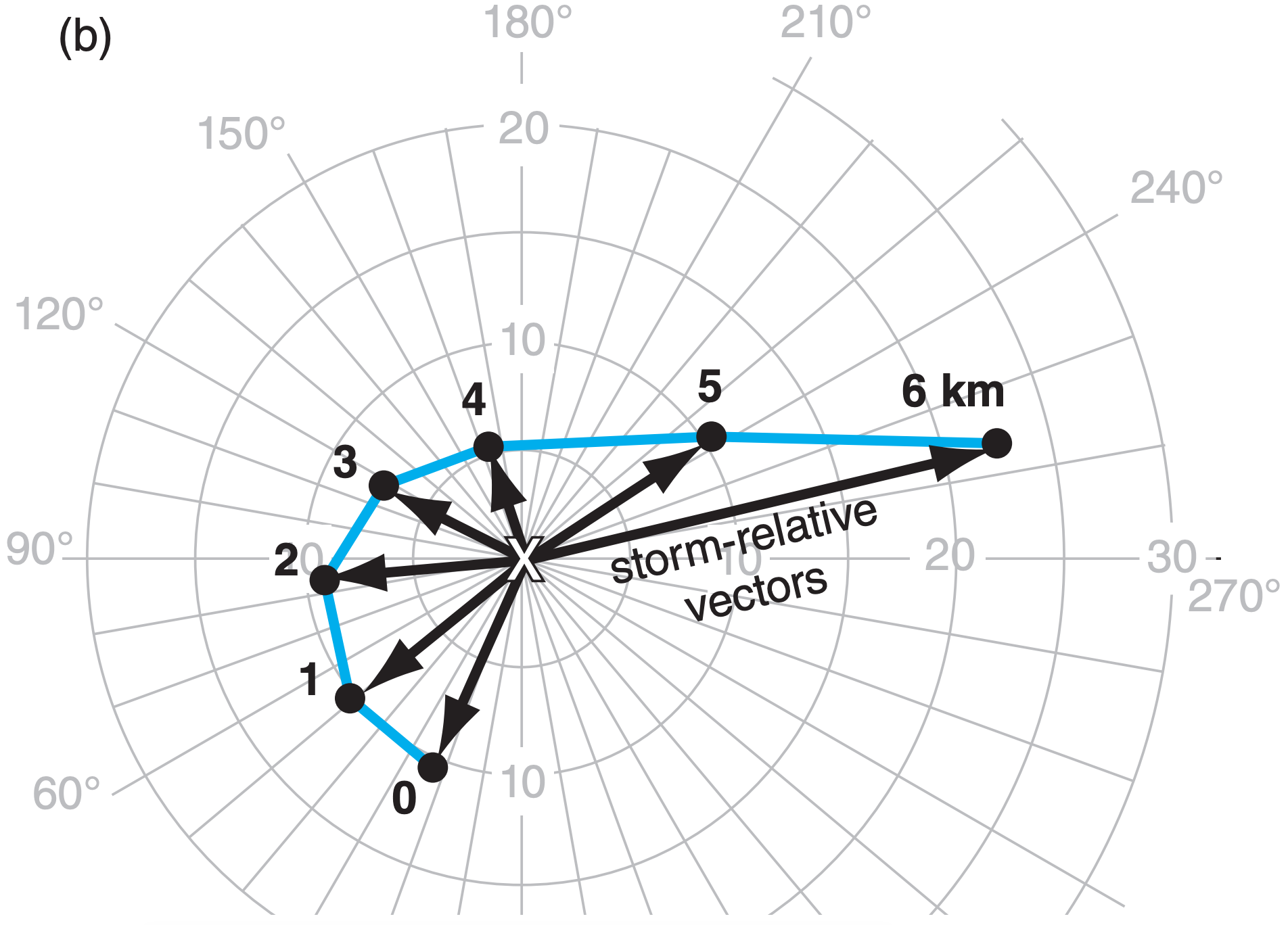
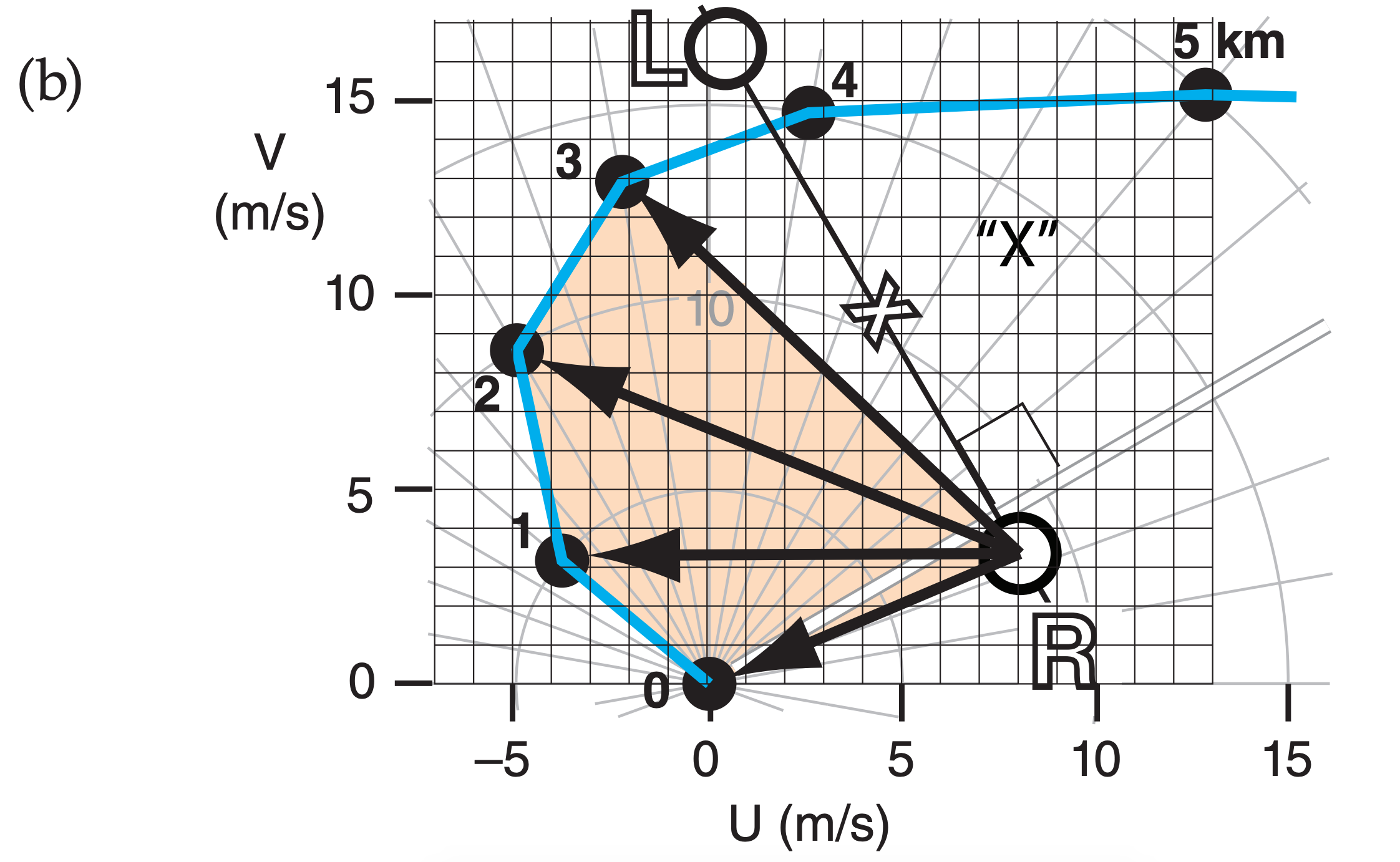
First, find the storm motion vector. If the thunderstorm already exists, then its motion can be tracked on radar or satellite (which gives a vector based on its actual speed and direction of movement). For forecasts of future thunderstorms, recall from the previous chapter that many thunderstorms move in the direction of the mean wind averaged over the 0 to 6 km layer of air, as indicated by the “X” in Fig. 15.40. Some supercell storms split into two parts: a right moving storm and a left moving storm, as was shown in the Thunderstorm Fundamentals chapter. Namely, if tornado formation from a right-moving supercell is of concern, then a mean storm vector associated with the “R” in Fig. 14.61 of the previous chapter should be used (i.e., do not use the “X”). See the Sample Application below, for an example.

Next, to find storm-relative winds, take the vector difference between the actual wind vectors and the storm-motion vector. On a hodograph, draw the storm-relative wind vectors from the storm-motion point to each of the original wind-profile data points. This is illustrated in Fig. 15.40a, based on the hodograph and normal storm motion “X”. After (optionally) repositioning the hodograph origin to coincide with the mean storm motion (Fig. 15.40b), the result shows the directions and speed of the storm-relative environmental wind vectors.

Figure 15.40 (a) Hodograph showing wind vector differences between the winds relative to a fixed-coordinate system (blue line hodograph) and the mean storm motion (X), based on the data from Figs. 14.57 & 14.59. (b) Same data, but with the hodograph origin shifted to “X” to give storm-relative wind vectors (black arrows). Some people find version (b) difficult to interpret, so they prefer to use version (a).

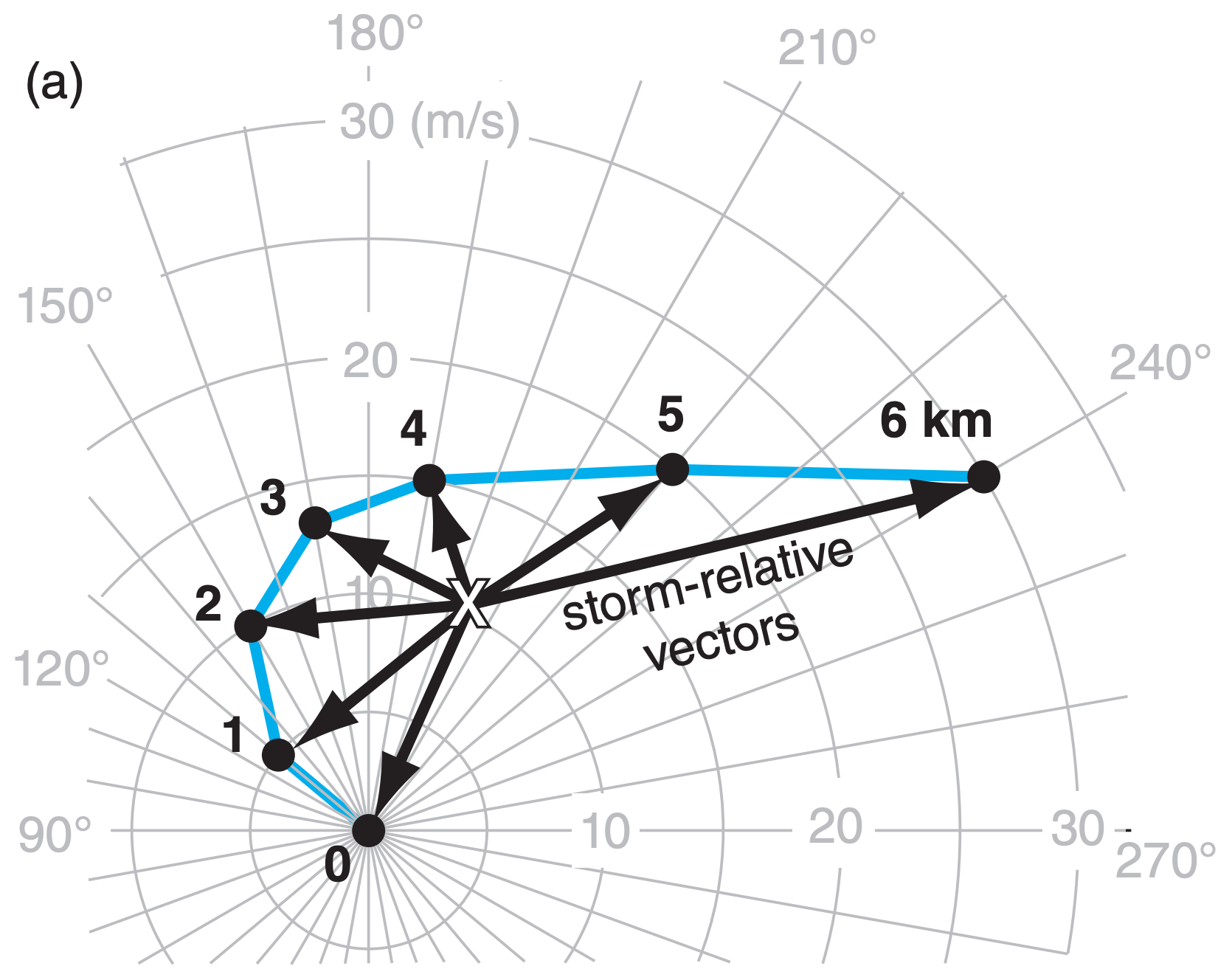
The algebraic components (U_j’, V_j’) and magnitude M’ of these storm-relative horizontal vectors are:

\(\ \begin{align} U_{j}^{\prime}=U_{j}-U_{s}\tag{15.49a}\end{align}\)

\(\ \begin{align} V_{j}^{\prime}=V_{j}-V_{s}\tag{15.49b}\end{align}\)

\(\ \begin{align} M_{j}^{\prime}=\left(U_{j}^{\prime 2}+V_{j}^{\prime 2}\right)^{1 / 2}\tag{15.50}\end{align}\)

where (U_j , V_j ) are the horizontal wind components at height index j, and the storm motion vector is (U_s, V_s). For a supercell that moves with the 0 to 6 km mean wind: (U_s, V_s) = \((\bar{U}, \bar{V})\) from the previous chapter. The vertical component of storm-relative winds W_j’ = W_j , because the thunderstorm does not translate vertically.

Most supercells have storm-relative winds of M’ = 7 to 10 m s^–1 at low altitudes [0 - 2 km above ground level (agl)] in the pre-storm environment. Environmental SR winds can also help you anticipate the type of supercell that might occur. Let M’_anvil be SR winds at the storm top (9 - 11 km agl).

• M’_anvil < 20 m s^–1 favors high-precipitation (HP) supercells
• 20 m s^–1 ≤ M’_anvil < 30 m s^–1 favors classic supercells
• 30 m s^–1 ≤ M’_anvil favors low-precipitation (LP) supercells

Sample Application

For the right-moving supercell of Fig. 14.61 from the previous chapter plot the storm-relative wind vectors on a hodograph.

Find the Answer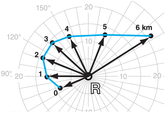

Given: Fig. 14.61. Storm motion indicated by “R”.

Find: Hodograph of storm-relative winds.

Method: Copy Fig. 14.61, draw relative vectors on it, and then re-center origin of hodograph to be at “R”:

Check: Similar to Fig. 15.40b.

Exposition: Compared to storm “X”, storm “R” has less directional shear, but more inflow at middle altitudes.

15.4.7. Origin of Tornadic Rotation

Because tornado rotation is around a vertical axis, this rotation can be expressed as a relative vertical vorticity ζr . Relative vorticity was defined in the General Circulation chapter as ζr =(∆V/∆x) – (∆U/∆y), and a forecast (tendency) equation for it was given in the Extratropical Cyclone chapter in the section on cyclone spin-up.

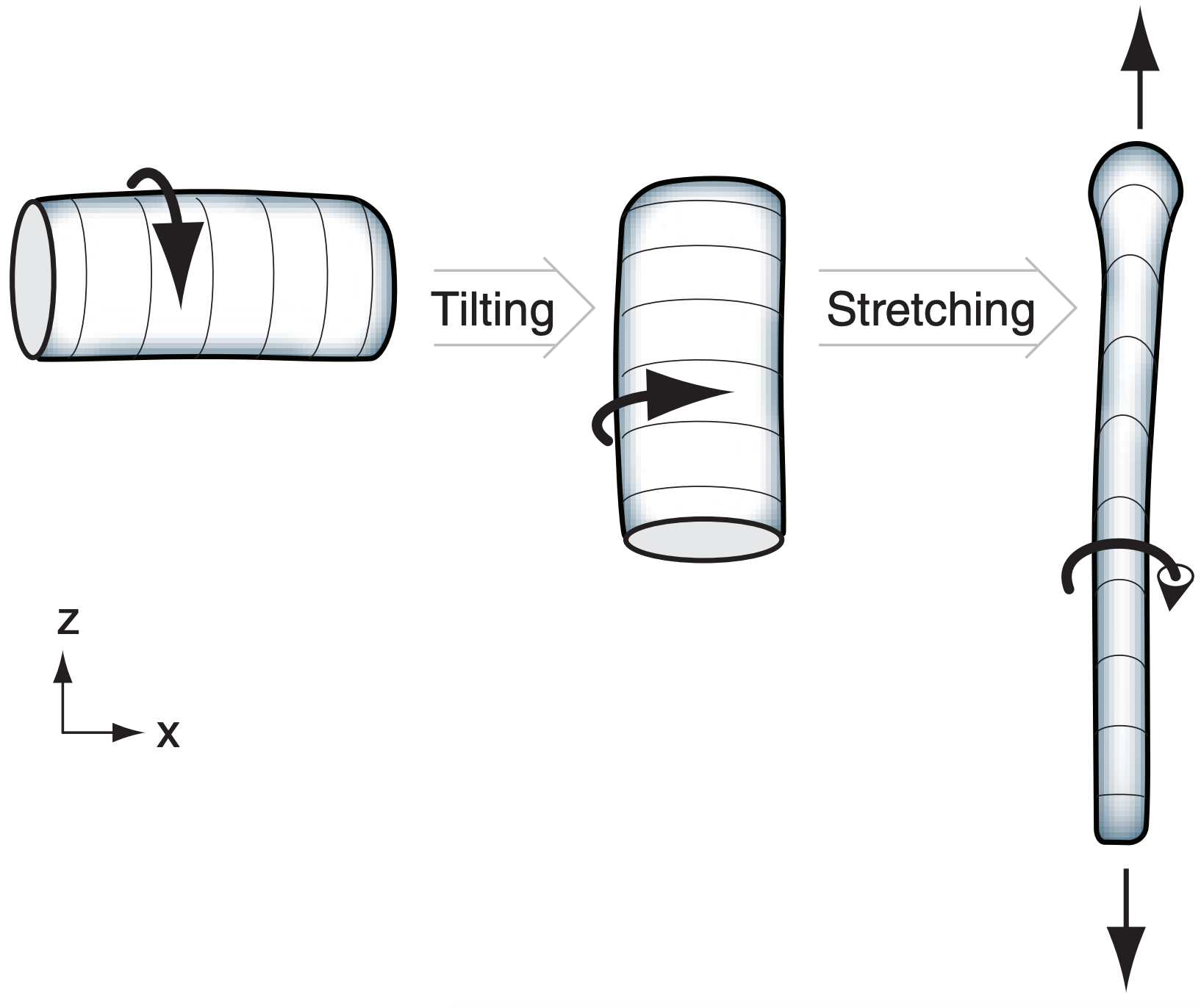
Relative to the thunderstorm, there is little horizontal or vertical advection of vertical vorticity, and the beta effect is small because any one storm moves across only a small range of latitudes during its lifetime. Thus, mesocyclone and tornadic vorticity are affected mainly by tilting, stretching, and turbulent drag:

\(\ \begin{align} \frac{\Delta \zeta_{r}}{\Delta t} \approx \frac{\Delta U^{\prime}}{\Delta z} \cdot \frac{\Delta W}{\Delta y}-\frac{\Delta V^{\prime}}{\Delta z} \cdot \frac{\Delta W}{\Delta x} +\left(\zeta_{r}+f_{c}\right) \cdot \frac{\Delta W}{\Delta z}-C_{d} \cdot \frac{M}{z_{T o r n B L}} \cdot \zeta_{r}\tag{15.51}\end{align}\)

\(\ \text{spin-up} \quad\quad \quad \quad \text{tilting} \quad \quad \quad\quad\quad\quad \quad \quad \text{stretching} \quad \quad \quad \text{turb.drag}\)

where the storm-relative wind components are (U’, V’, W), the Coriolis parameter is f_c, the tangential wind speed is approximately M, drag coefficient is C_d, and z_TornBL is the depth of the tornado’s boundary layer (roughly 100 m).

This simplified vorticity-tendency equation says that rotation about a vertical axis can increase (i.e., spin up) if horizontal vorticity is tilted into the vertical, or if the volume of air containing this vertical vorticity is stretched in the vertical (Fig. 15.41). Also, cyclonically-rotating tornadoes (namely, rotating in the same direction as the Earth’s rotation, and having positive ζr) are favored slightly, due to the Coriolis parameter in the stretching term. Rotation decreases due to turbulent drag, which is greatest at the ground in the tornado’s boundary layer.

Figure 15.41 Tilting can change rotation about a horizontal axis to rotation about a vertical axis, to create a mesocyclone (a rotating thunderstorm). Stretching can then intensify the rotation into a tornado.

Most theories for tornadic rotation invoke tilting and/or stretching of vorticity, but these theories disagree about the origin of rotation. There is some evidence that different mechanisms might trigger different tornadoes.

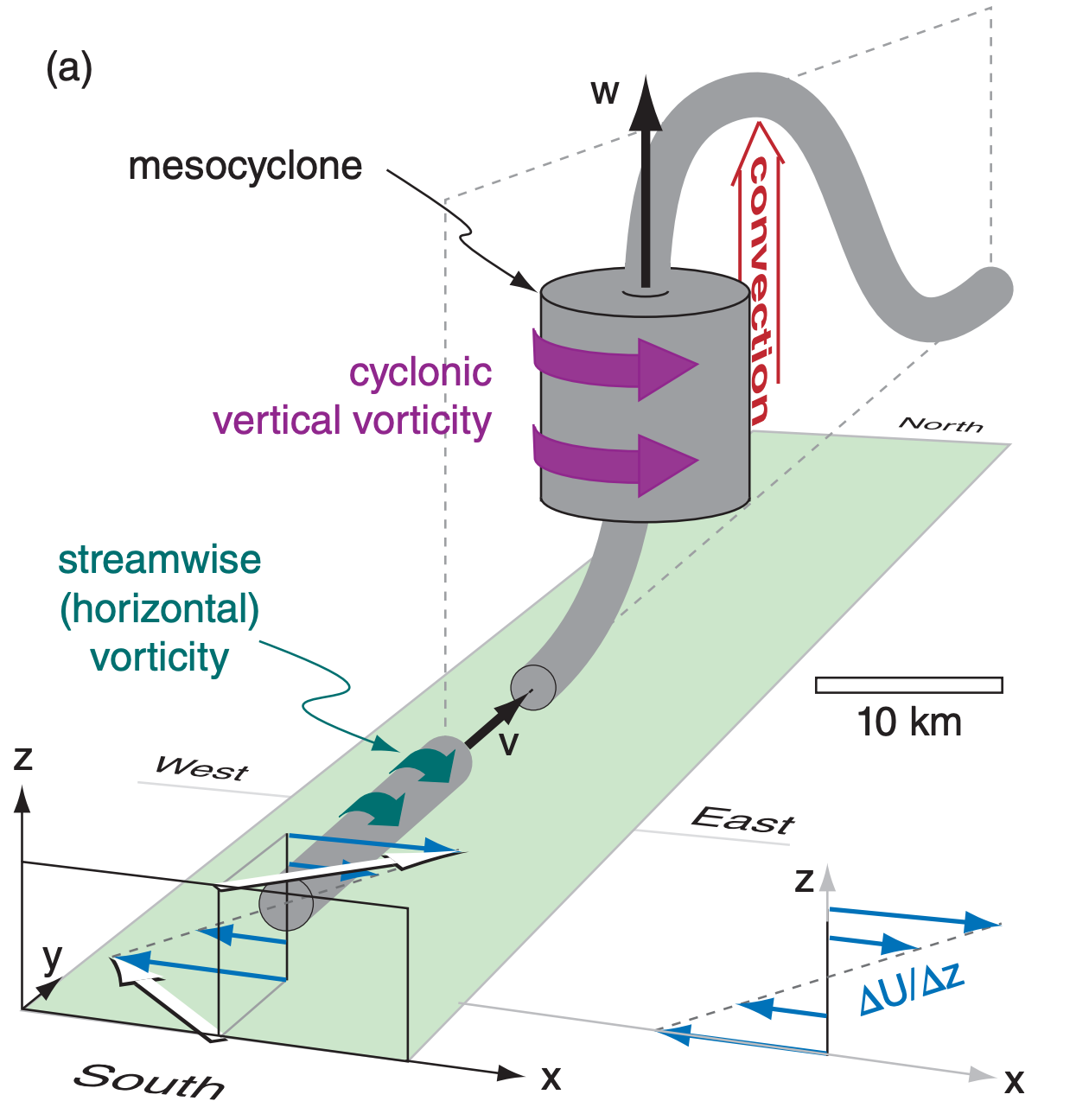
Two theories focus on rotation about a horizontal axis in the atmospheric boundary layer. One theory suggests that streamwise vorticity (rotation about a horizontal axis aligned with the mean wind direction) exists in ambient (outside-of-the-storm) air due to vertical shear of the horizontal wind ∆U/∆z in Fig. 15.42a. Once this air reaches the inflow region of the thunderstorm, the horizontal streamwise vorticity is tilted by convective updrafts to create rotation around a vertical axis.

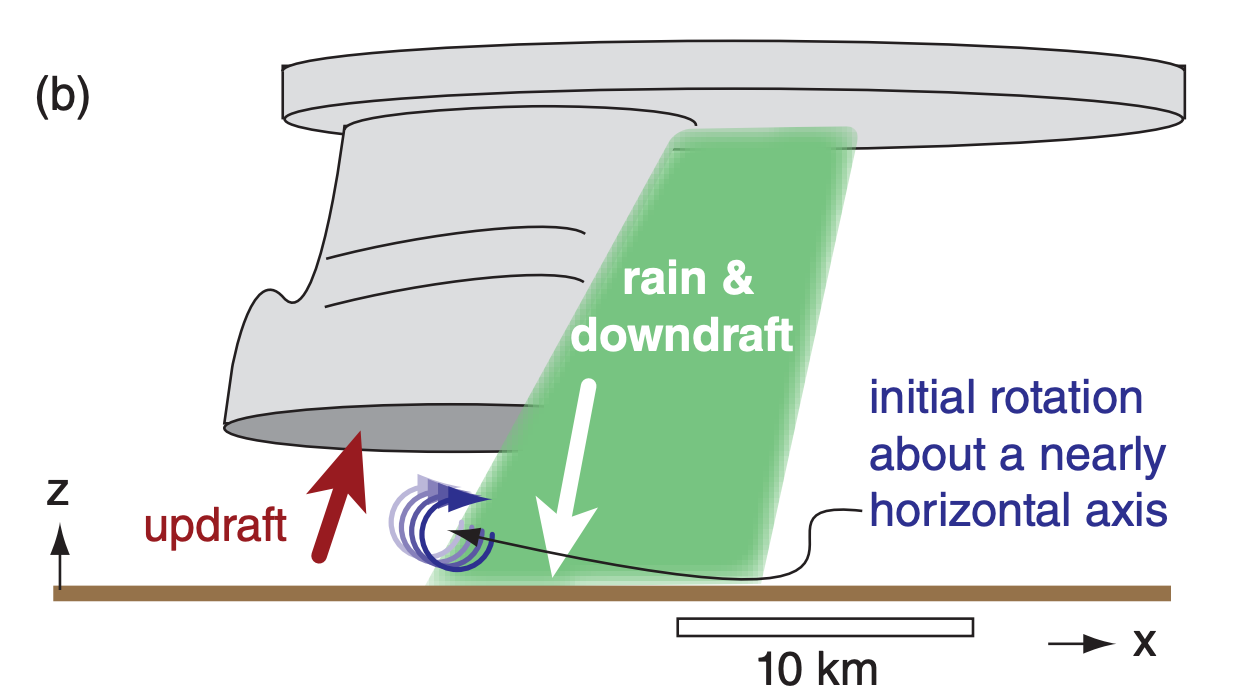
Another theory considers shears in vertical velocity that develop near the ground where cool precipitation-induced downdrafts are adjacent to warm updrafts. The result is vorticity about a nearly horizontal axis (Fig. 15.42b), which can be tilted towards vertical by the downdraft air near the ground.

Figure 15.42 Theories for creation of initial rotation about a horizontal axis. (a) Vertical shear of the horizontal wind (∆U/∆z) causes streamwise horizontal vorticity (dark slender horizontal cylinder), which can be tilted by convective updrafts to create mesocyclones (fat vertical cylinder). This wind profile is typical of the prairies in central North America. (b) Shear between thunderstorm downdraft and updraft creates rotation close to the ground with a horiz. axis that can be tilted to vertical.

Two other theories utilize thunderstorm updrafts to stretch existing cyclonic vertical vorticity. One suggests that the precipitation-cooled downdraft will advect the mesocyclone base downward, thereby stretching the vortex and causing it to spin faster. Such a mechanism could apply to mesoscale convective vortices (MCVs) in the mid troposphere. The other theory considers thunderstorm updrafts that advect the top of the mesocyclone upward — also causing stretching and spin-up.

Another theory suggests that large-scale rotation about a vertical axis of a synoptic-scale cyclone can cascade down to medium (mesocyclone) scales and finally down to small (tornadic) scales. All of these previous theories are for supercell tornadoes.

Weaker tornadoes are suggested to form at boundaries between cold and warm airmasses near the ground. The cold airmass could be the result of precipitation-cooled air that creates a downburst and associated outflow winds. At the airmass boundary, such as a cold front or gust front, cold winds on one side of the boundary have an along-boundary component in one direction while the warmer winds on the other side have an along-boundary component in the opposite direction. The vertical vorticity associated with these shears (∆U/∆y and ∆V/∆x) can be stretched to create landspouts and gustnadoes.

15.4.8. Helicity

Many of the previous theories require a mesocyclone that has both rotation and updraft (Fig. 15.43a). The combination of these motions describes a helix (Fig. 15.43b), similar to the shape of a corkscrew.

Figure 15.43 (a) Sketch of a supercell thunderstorm showing both mesocyclone rotation (yellow arrow) and updraft (black arrow). (b) Cross-section showing helical motions (yellow arrows) in the mesocyclone and smaller-diameter but faster rotation of the tornado vortex (dark-blue helix). ζr is relative vorticity, and w is vertical velocity.

Define a scalar variable called helicity, H, at any one point in the air that combines rotation around some axis with mean motion along the same axis:

\(\ \begin{align} H=U_{a v g} & \cdot\left[\frac{\Delta W}{\Delta y}-\frac{\Delta V}{\Delta z}\right]+V_{a v g} \cdot\left[-\frac{\Delta W}{\Delta x}+\frac{\Delta U}{\Delta z}\right]+ W_{a v g} \cdot\left[\frac{\Delta V}{\Delta x}-\frac{\Delta U}{\Delta y}\right] \tag{15.52}\end{align}\)

where U_avg = 0.5·(U_j+1 + U_j ) is the average U-component of wind speed between height indices j and j+1. V_avg and Wavg are similar. ∆U/∆z = (U_j+1 – U_j )/ (z_j+1 –z_j ), and ∆V/∆z and ∆W/∆z are similar. Helicity units are m·s^–2, and the differences ∆ should be across very small distances.

If the ambient environment outside the thunderstorm has only vertical shear of horizontal winds, then eq. (15.52) can be simplified to be:

\(\ \begin{align} H \approx V_{a v g} \cdot \frac{\Delta U}{\Delta z}-U_{a v g} \cdot \frac{\Delta V}{\Delta z}\tag{15.53}\end{align}\)

which gives only streamwise-vorticity contribution to the total helicity. Alternatively, if there is only rotation about a vertical axis, then eq. (15.52) can be simplified to give the vertical-relative-vorticity ζr contribution to total helicity:

\(\ \begin{align} H=W_{a v g} \cdot\left[\frac{\Delta V}{\Delta x}-\frac{\Delta U}{\Delta y}\right]=W_{a v g} \cdot \zeta_{r}\tag{15.54}\end{align}\)

If helicity H is preserved while thunderstorm upand down-drafts tilt the streamwise vorticity into vertical vorticity, then you can equate the H values in eqs. (15.53) and (15.54). This allows you to forecast mesocyclone rotation for any given shear in the pre-storm environment. Greater values of streamwise helicity in the environment could increase the relative vorticity of a mesocyclone, making it more tornadogenic (tending to spawn new tornadoes).

Sample Application

(a) Given the velocity sounding below, what is the associated streamwise helicity?

z (km)	U (m s^–1)	V (m s^–1)
1	1	7
2	5	9

(b) If a convective updraft of 12 m s–1 tilts the streamwise vorticity from (a) into the vertical while preserving its helicity, what is the vertical vorticity value?

Find the Answer

Given: (a) in the table above (b) w = 12 m s^–1

Find: (a) H = ? m·s^–2 (b) ζr = ? s^–1

(a) First find the average wind between the two given heights [U_avg=(1+5)/2 = 3 m s^–1. Similarly V_avg = 8 m s^–1]. Then use eq. (15.53):

\(\begin{aligned} H \approx &(8 \mathrm{m} / \mathrm{s}) \cdot \frac{(5-1 \mathrm{m} / \mathrm{s})}{(2000-1000 \mathrm{m})}-(3 \mathrm{m} / \mathrm{s}) \cdot \frac{(9-7 \mathrm{m} / \mathrm{s})}{(2000-1000 \mathrm{m})} \\ &=0.032+0.006 \mathrm{m} \cdot \mathrm{s}^{-2}=\underline{\mathbf{0.038 \mathrm{m} \cdot \mathrm{s}^{-2}}} \end{aligned}\)

(b) Use this helicity in eq. (15.54):

(0.038 m·s^–2) = (12m·s^–1) · ζr . Thus, ζr = 0.0032 s^–1

Check: Physics & units OK.

Exposition: Time lapse photos of mesocyclones show rotation about 100 times faster than for synoptic lows.

More useful for mesocyclone and tornado forecasting is a storm relative helicity (SRH), which uses storm-relative environmental winds (U’, V’) to get a relative horizontal helicity contribution H’. Substituting storm-relative winds into eq. (15.53) gives:

\(\ \begin{align} H^{\prime} \approx V_{a v g}^{\prime} \cdot \frac{\Delta U^{\prime}}{\Delta z}-U_{a v g}^{\prime} \cdot \frac{\Delta V^{\prime}}{\Delta z}\tag{15.55}\end{align}\)

where U’_avg = 0.5·(U’_j+1 + U’_j ) is the average U’-component of wind within the layer of air between height indices j and j+1, and V’_avg is found similarly.

To get the overall effect on the thunderstorm, SRH then sums H’ over all atmospheric layers within the inflow region to the thunderstorm, multiplied by the thickness of each of those layers.

\(\ \begin{align} S R H \quad=\sum H^{\prime} \cdot \Delta z\tag{15.56}\end{align}\)

\(\ \begin{align} =\sum_{j=0}^{N-1}\left[\left(V_{j}^{\prime} \cdot U_{j+1}^{\prime}\right)-\left(U_{j}^{\prime} \cdot V_{j+1}^{\prime}\right)\right]\tag{15.57}\end{align}\)

where N is the number of layers, j = 0 is the bottom wind-observation index (usually at the ground, z = 0), and j = N is the top wind-observation index (at the top of the inflow region). Normally, the inflow region spans all atmospheric layers from the ground to 1 or 3 km altitude. Units of SRH are m²·s^–2.

On a hodograph, the SRH is twice the area swept by the storm-relative wind vectors in the inflow region (Fig. 15.44).

Figure 15.44 Storm-relative helicity (SRH) between the surface and z = 3 km is twice the shaded area. But for any hodograph, you will likely get different areas for normal, left-moving, and right-moving storms. (a) For “normal” storm motion “X”, based on hodograph of Figs. 14.61 & 15.40a. (b) For right-moving storm motion “R”, based on the hodograph of Fig. 14.61.

In computer-simulated storms, an updraft helicity is defined as UH = ∑(W·ζr·∆z), where the sum is over layers (each of thickness ∆z) between 2 & 5 km altitude agl. UH units are m²·s^–2, similar to SRH.

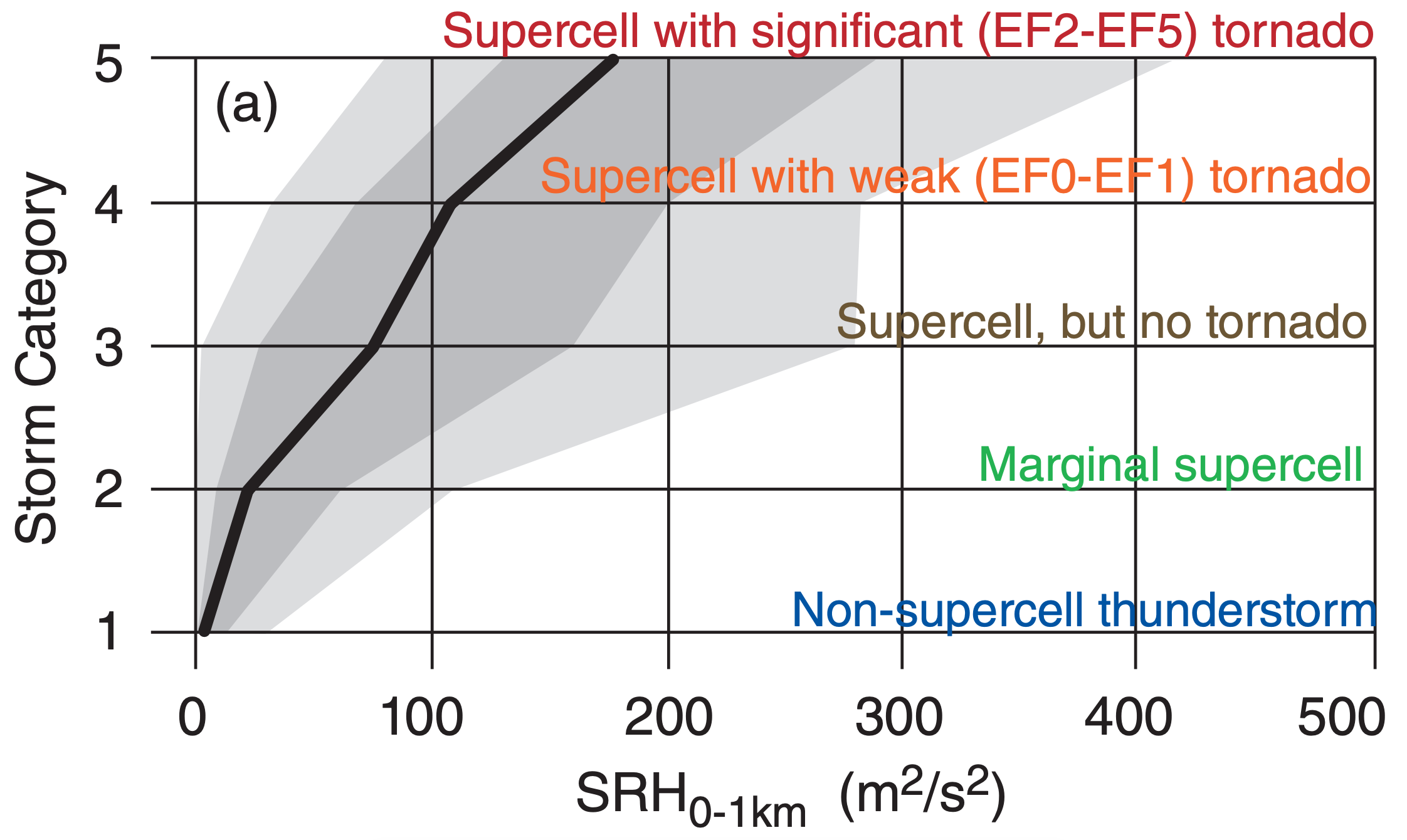
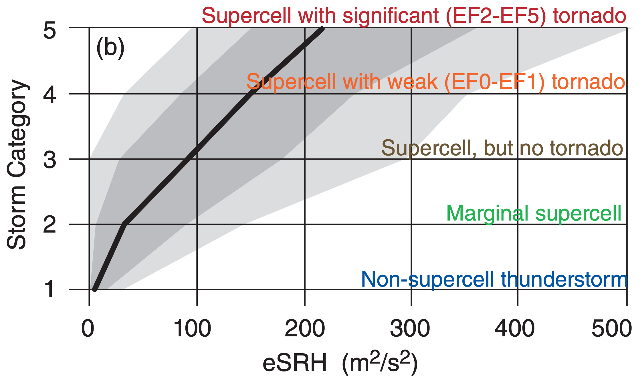
SRH is an imperfect indicator of whether thunderstorms are likely to be supercells and form tornadoes, hail, and strong straight-line winds. Fig. 15.45 shows the relationship between SRH values and tornado strength. Some evidence suggests that the 0 to 1 km SRH (Fig. 15.46) is a slightly better indicator than SRH over the 0 to 3 km layer.

Figure 15.45 Approximate relationship between storm-relative helicity (SRH) and tornado strength on the Enhanced Fujita scale (EF0 to EF5), for North America. “Supercell” indicates a non-tornadic mesocyclonic thunderstorm. Caution: the shaded domain boundaries are not as sharp as drawn. Solid and dashed lines are medians.

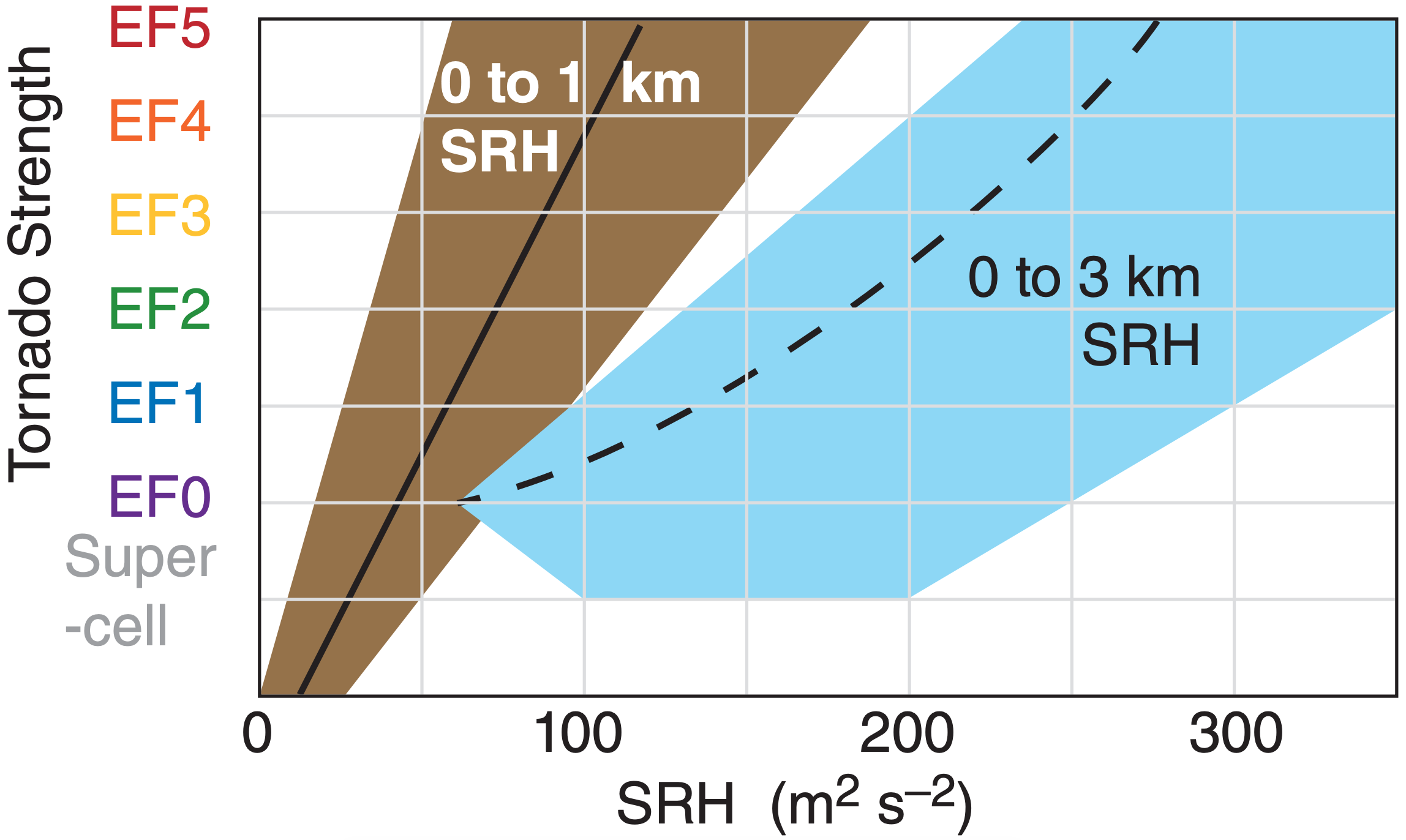
One difficulty with SRH is its sensitivity to storm motion. For example, hodographs of veering wind as plotted in Fig. 15.44 would indicate much greater SRH for a right moving (“R”) storm compared to a supercell that moves with the average 0 to 6 km winds (“X”). For this reason, observed storm motion give better SRH estimates than predicted motion.

Sample Application

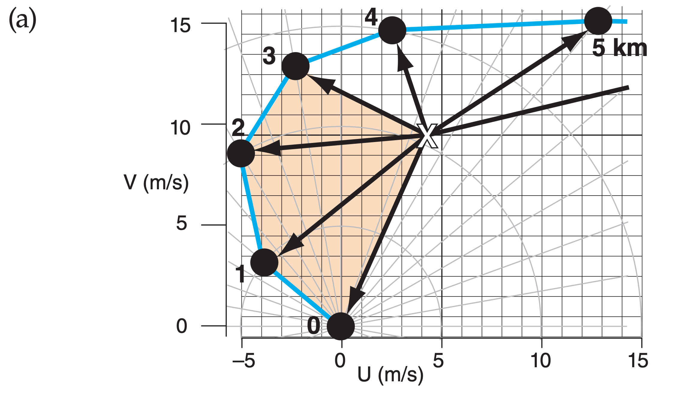
For the hodograph of Fig. 15.44a, graphically find SRH for the (a) z = 0 to 3 km layer, and (b) 0 to 1 km layer. (c, d) Find the SRHs for those two depths using an equation method. (e) Discuss the potential for tornadoes?

Find the Answer

Given Fig. 15.44a.

Find: 0-3 km & 0-1 km SRH = ? m²·s^–2 , both graphically & by eq.

a) Graphical method: Fig. 15.44a is copied below, and zoomed into the shaded region. Count squares in the shaded region of the fig., knowing that each square is 1 m s^–1 by 1 m s^–1, and thus spans 1 m²·s^–2 of area.

When counting squares, if a shaded area (such as for square #2 in the fig. below) does not coverthe whole square, then try to compensate with other portions of shaded areas (such as the small shaded triangle just to the right of square #2).

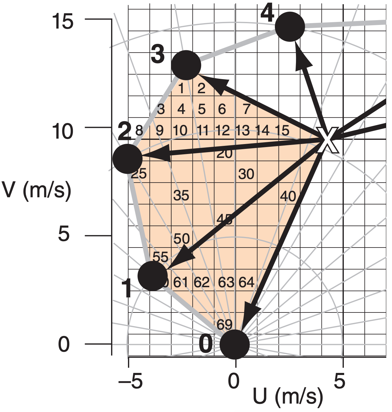
Thus, for 0 to 3 km SRH:

SRH = 2·(# of squares)·(area of each square)

SRH =2 · (69 squares) · (1 m²·s^–2/square) = 138 m²·s^–2.

b) For 0 to 1 km: SRH:

SRH =2 · (25 squares) · (1 m²·s^–2/square) = 50 m²·s^–2.

c) Equation method: Use eq. (15.57). For our hodograph, each layer happens to be 1 km thick. Thus, the index j happens to correspond to the altitude in km of each wind observation, for this fortuitous situation.

For the 0-3 km depth, eq. (15.57) expands to be:

SRH	= V’0 · U’1 – U’0 · V’1	(for 0 ≤ z ≤ 1 km)
	+ V’1 · U’2 – U’1 · V’2	(for 1 ≤ z ≤ 2 km)
	+ V’2 · U’3 – U’2 · V’3	(for 2 ≤ z ≤ 3 km)

Because the figure at left shows storm-relative winds, we can pick off the (U’, V’) values by eye at each level:

z (km)	U’ (m s^–1)	V’ (m s^-1)
0	–4.3	–9.5
1	–8.1	–6.2
2	–9.3	–1.0
3	–7.7	+3.3

Plugging these values into the eq. above gives:

\(\begin{aligned} \mathrm{SRH} &=(-9.5) \cdot(-8.1)-(-4.3) \cdot(-6.2) \\ &+(-6.2) \cdot(-9.3)-(-8.1) \cdot(-1.0) \\ &+(-1.0) \cdot(-7.7)-(-9.3) \cdot(+3.3) \\ \mathrm{SRH} &=76.95-26.66+57.66-8.1+7.7+30.69 \\ &=\mathbf{1 3 8 . 2 \mathrm{m}^{2} \cdot \mathrm{s}^{-2}} \text {for } 0-3 \mathrm{km} \end{aligned}\)

d) 0-1 km SRH = 76.95 – 26.66 = 50.3 m²·s^–2 .

e) Using Fig. 15.45 there is a good chance of supercells and EF0 to EF1 tornadoes. Slight chance of EF2 tornado. However, Fig. 15.46 suggests a supercell with no tornado.

Check: Units OK. Physics OK. Magnitudes OK.

Exposition: The graphical and equation methods agree amazingly well with each other. This gives us confidence to use either method, whichever is easiest.

The disagreement in tornado potential between the 0-1 and 0-3 km SRH methods reflects the tremendous difficulty in thunderstorm and tornado forecasting. Operational meteorologists often must make difficult decisions quickly using conflicting indices.

INFO • Effective Inflow Layer for SRH

Consider the nighttime sounding plotted on the emagram in Fig. (a) below. An air parcel (filled and open circles representing T and T_d, respectively) lifted from 100 kPa would have very large CIN magnitude but no CAPE. Thus, cold air from 100 kPa would NOT likely be drawn into a thunderstorm.

An air parcel starting at 90 kPa from the same sounding (Fig. b) would have positive CAPE and small CIN. This is likely within the effective inflow layer, and is typical of a residual layer above a stable layer.

But the parcel starting from 80 kPa in Fig. (c) would not likely be in the effective inflow layer, because the CIN has greater magnitude but CAPE is weaker.

Computer programs can automatically test many more starting altitudes to pinpoint the effective inflow layer.

Figure 15.46 Statistics of thunderstorm intensity vs. (a) storm-relative helicity (SRH) across a 0 to 1 km fixed-layer of air; and (b) effective storm-relative helicity (eSRH). For several hundred storms in central N. America, the black line is the median (50 percentile); dark grey shading spans 25^th to 75^th percentiles (the interquartile range); and light grey spans 10^th to 90^th percentiles.

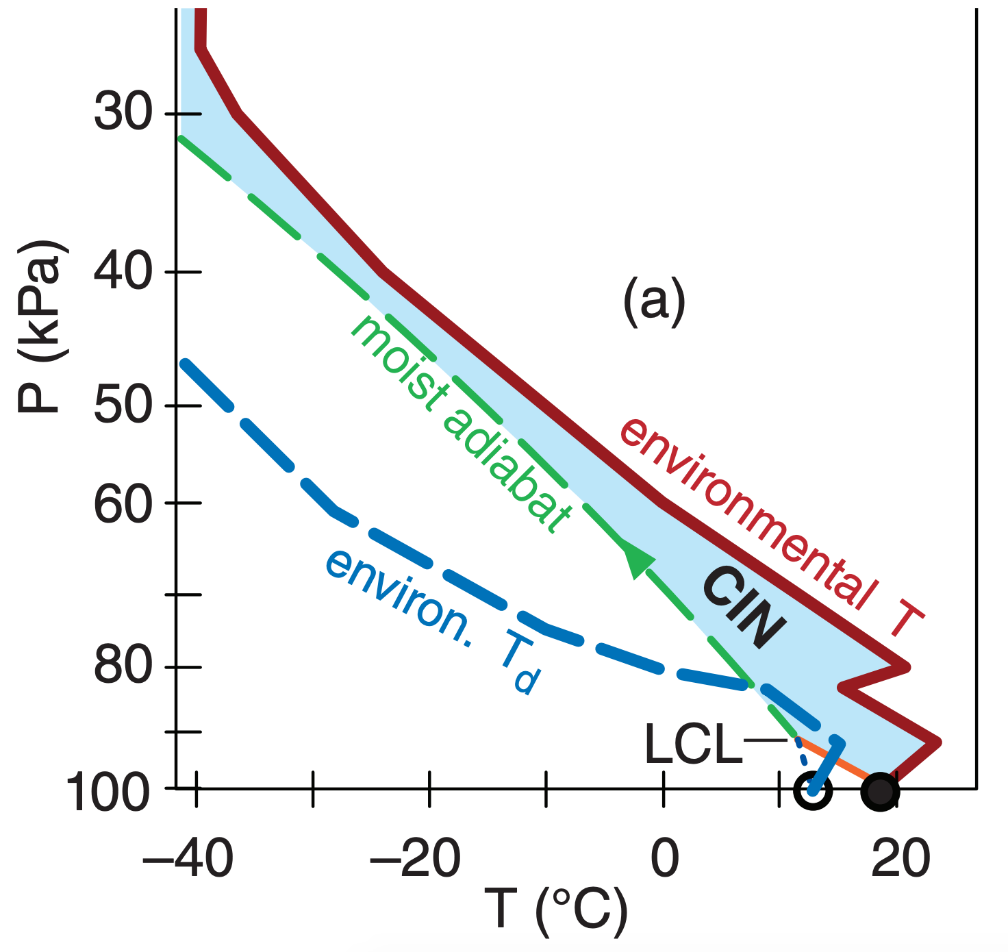
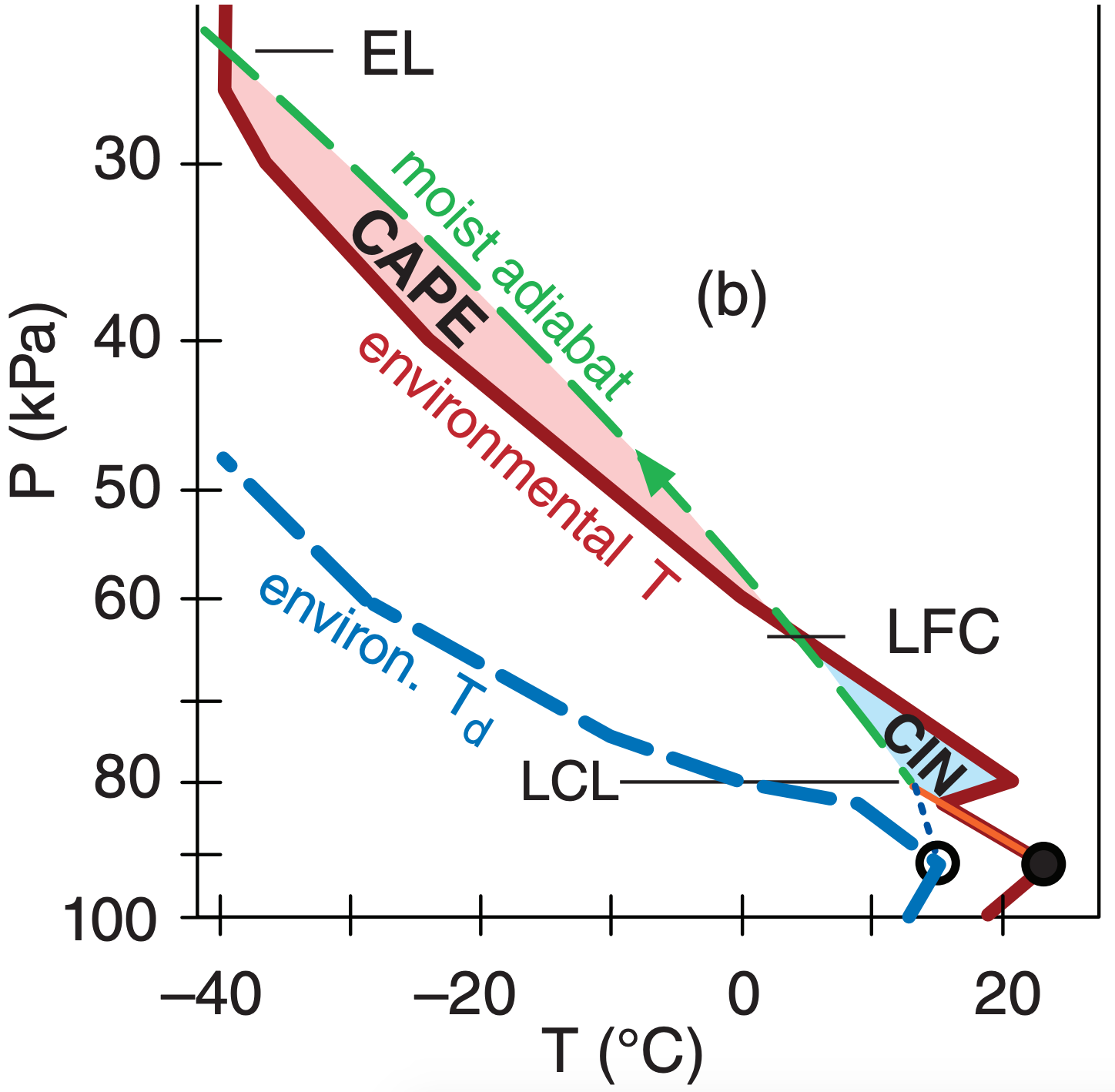
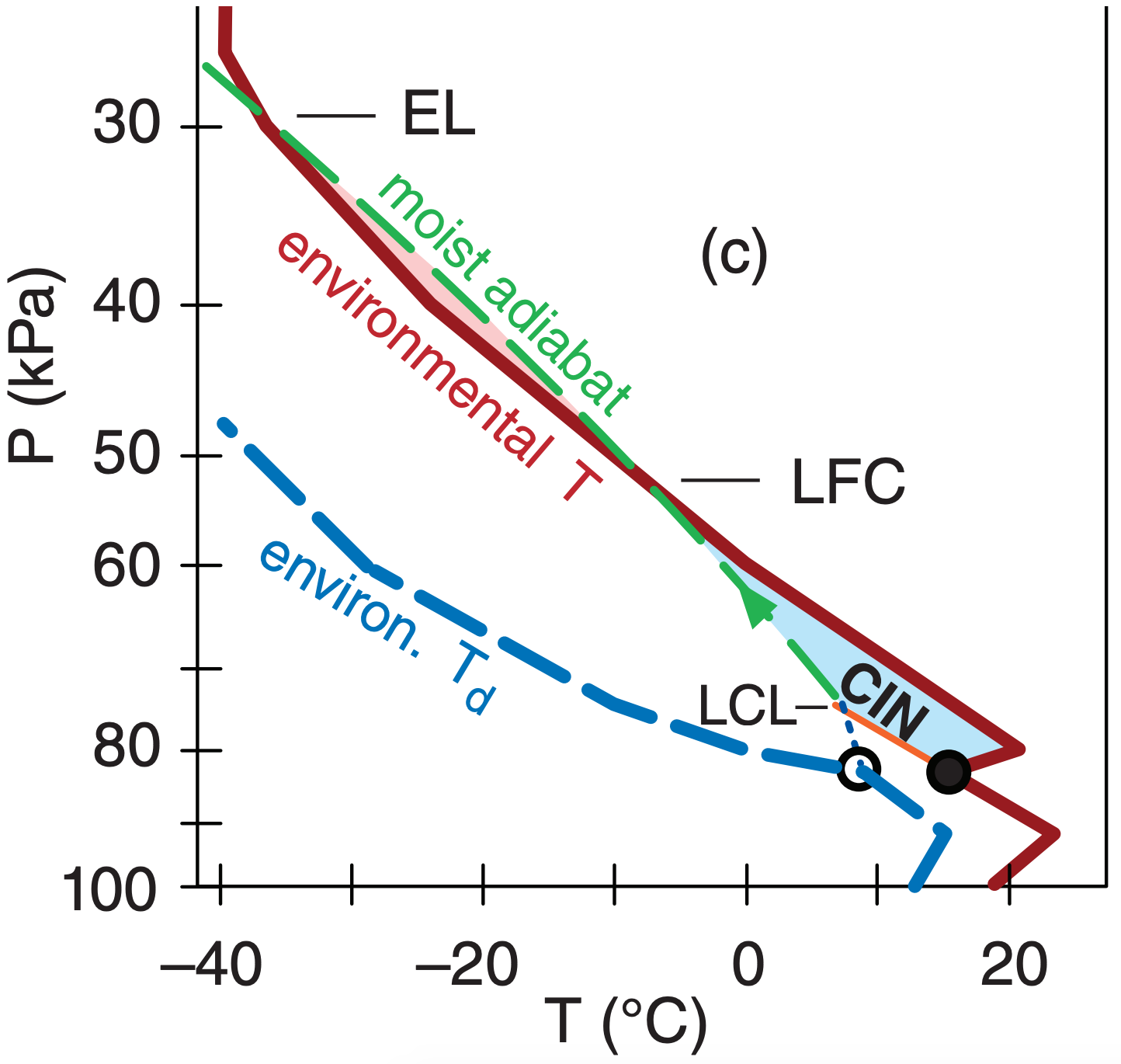
Because thunderstorms do not necessarily draw in air from the 0 to 1 km layer, an effective Storm Relative Helicity (eSRH) has been proposed that is calculated across a range of altitudes that depends on CAPE and CIN of the environmental sounding. The bottom altitude, called the effective-inflow base, is found as the lowest starting altitude for a rising air parcel that satisfies two constraints: CAPE ≥ 100 J kg^–1 when lifted to its EL, and CIN ≥ –250 J kg^–1 (i.e., is less negative than –250 J kg^–1). The top altitude of the effective inflow layer is the lowest starting height (above the inflow base) for which rising air-parcel CAPE ≤ 100 J kg^–1 or CIN ≤ –250 J kg^–1. The INFO box at left illustrates this concept.

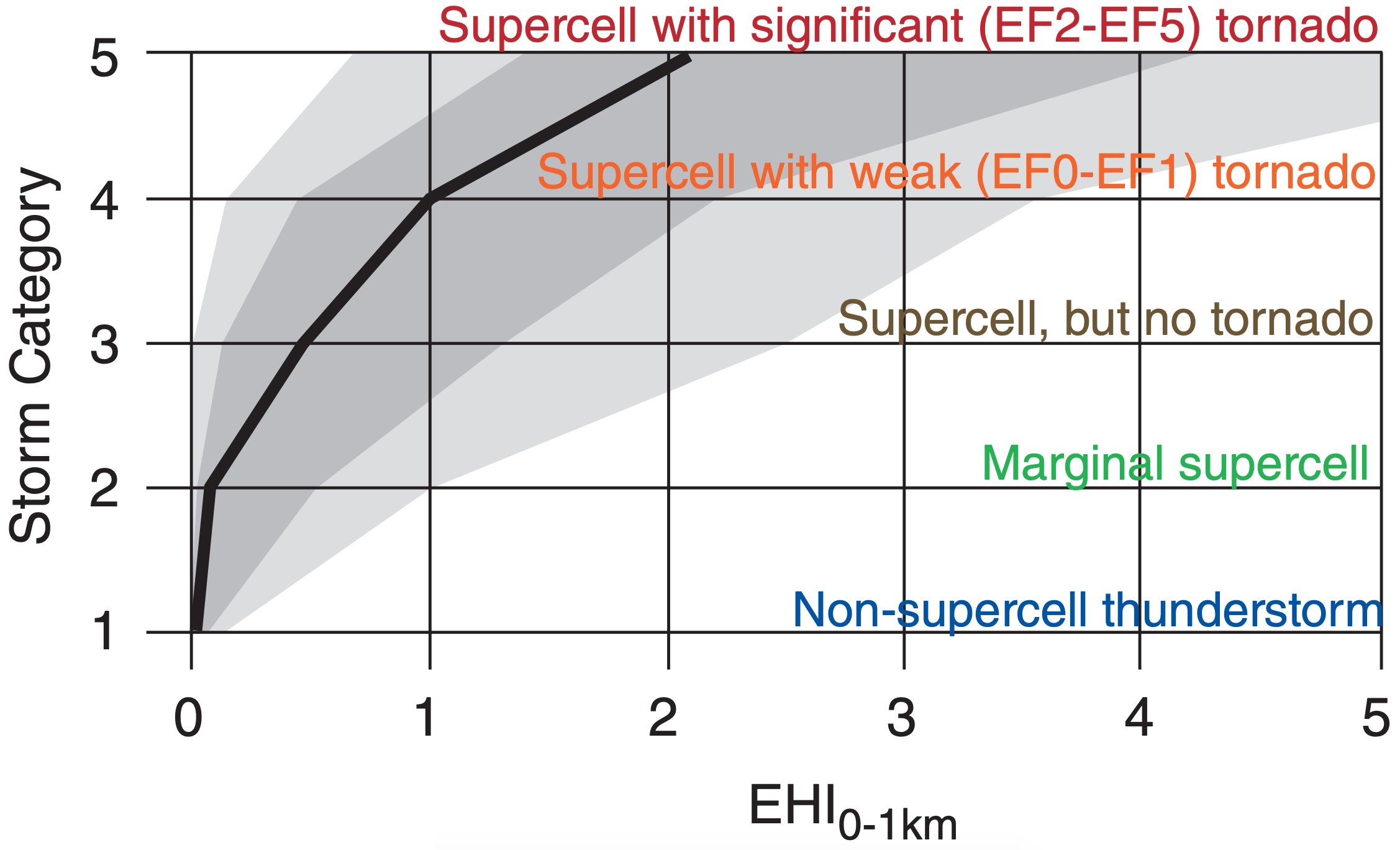
The eSRH calculation is made only if the top and bottom layer altitudes are within the bottom 3 km of the atmosphere. eSRH is easily found using computer programs. Fig. 15.47 shows a map of eSRH for the 24 May 2006 case.

Figure 15.47 A case-study example of effective storm-relative helicity (eSRH) in units of m² s^–2 at 23 UTC on 24 May 2006, over the USA. Values of eSRH greater than 200 m² s^–2 are shaded, and indicate locations of greatest likelihood for tornadic supercells.

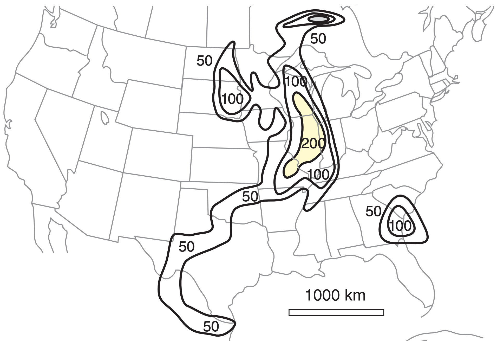
Fig. 15.46b shows that eSRH better discriminates between non-tornadic and tornadic supercells than SRH. eSRH works even if the storm ingests residual-layer air that lies on top of a shallow stable layer of colder air, such as occurs at night, as illustrated in the INFO box at left.

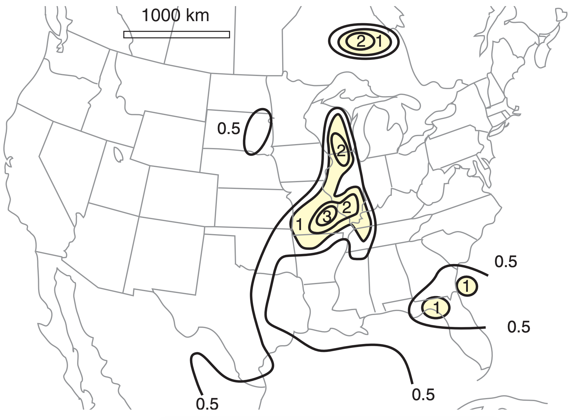
As sketched in Fig. 15.43a, both updraft and rotation (vorticity) are important for mesocyclone formation. You might anticipate that the most violent supercells have both large CAPE (suggesting strong updrafts) and large SRH (suggesting strong rotation). A composite index called the Energy Helicity Index (EHI) combines these two variables:

\(\ \begin{align} E H I=\frac{C A P E \cdot S R H}{a}\tag{15.58}\end{align}\)

where a = 1.6x10⁵ m⁴·s^–4 is an arbitrary constant designed to make EHI dimensionless and to scale its values to lie between 0 and 5 or so. Large values of EHI suggest stronger supercells and tornadoes.

CAPE values used in EHI are always the positive area on the thermo diagram between the LFC and the EL. MLCAPE SRH values can be either for the 0 to 1 km layer in the hodograph, or for the 0 to 3 km layer. For this reason, EHI is often classified as 0-1 km EHI or 0-3 km EHI. Also, EHI can be found either from actual rawinsonde observations, or from forecast soundings extracted from numerical weather prediction models. An effective energy helicity index (eEHI) can also be calculated from eSRH.

Table 15-5. Energy Helicity Index (0-3 km EHI) as an indicator of possible tornado existence and strength.
EHI	Tornado Likelihood
< 1.0	Tornadoes & supercells unlikely.
1.0 to 2.0	Supercells with weak, short-lived tornadoes possible. Non-supercell tornadoes possible (such as near bow echoes).
2.0 to 2.5	Supercells likely. Mesocyclone-induced tornadoes possible.
2.5 to 3.0	Mesocyclone-induced supercell tornadoes more likely.
3.0 to 4.0	Strong mesocyclone-induced tornadoes (EF2 and EF3) possible.
> 4.0	Violent mesocyclone-induced tornadoes (EF4 and EF5) possible.

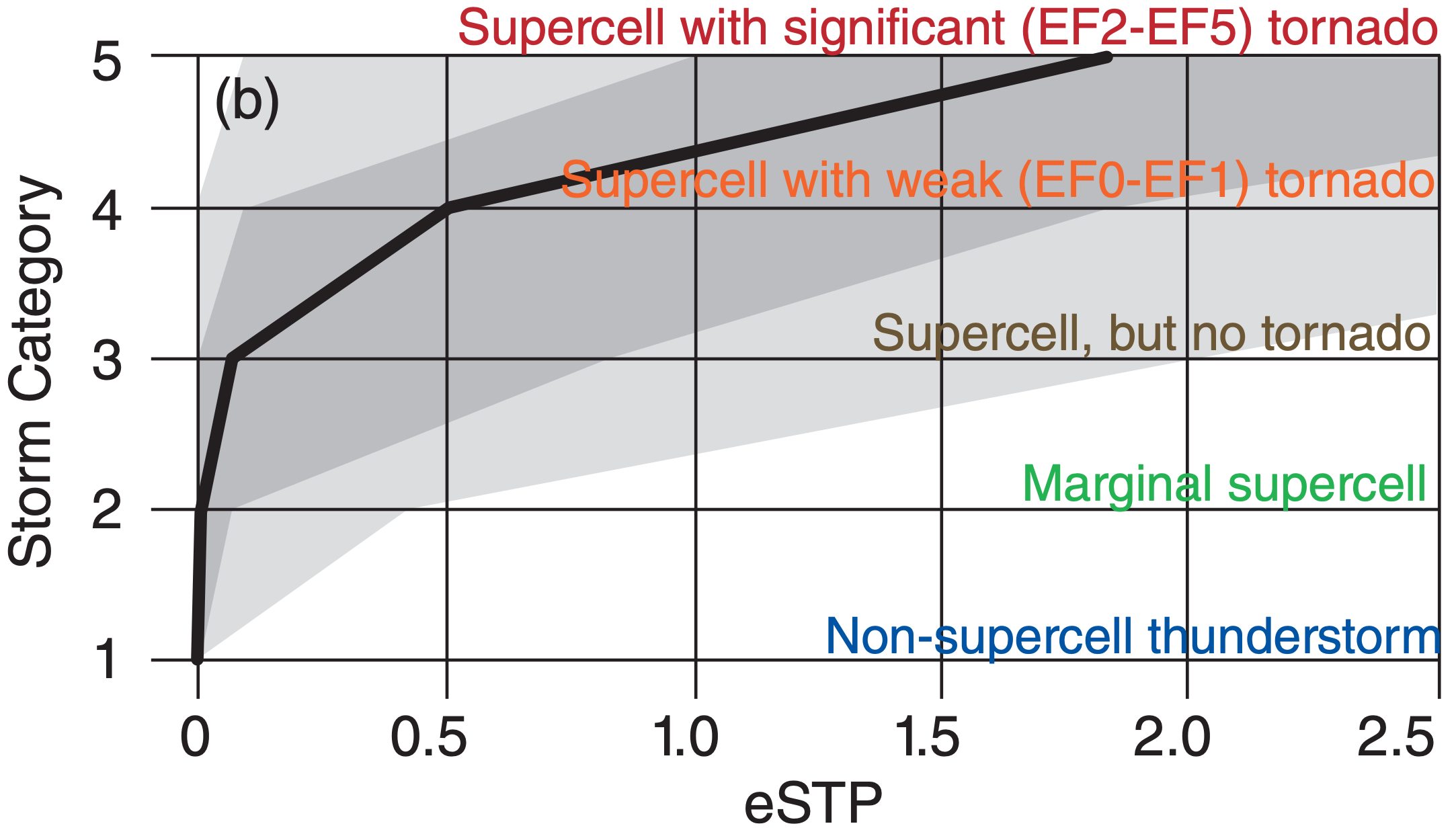
Table 15-5 indicates likely tornado strength in North America as a function of 0-3 km EHI. Caution: the EHI ranges listed in this table are only approximate. If 0-1 km EHI is used instead, then significant tornadoes can occur for EHI as low as 1 or 2, such as shown in Fig. 15.48. To illustrate EHI, Fig. 15.49 shows a forecast weather map of EHI for 24 May 2006.

Figure 15.48 Statistics of thunderstorm intensity vs. energy helicity index (EHI) across a 0 to 1 km layer of air. For several hundred storms in central N. America, the black line is the median (50 percentile); dark grey shading spans 25^th to 75^th percentiles (the interquartile range); and light grey spans 10^th to 90^th percentiles.

Figure 15.49 Map of energy helicity index (EHI) over the 0 to 1 km layer, for the 23 UTC case on 24 May 2006, over the USA. Dimensionless values greater than 1 are shaded, and suggest stronger supercell storms with greater likelihood of tornadoes.

Sample Application

Suppose a prestorm sounding shows that the convective available potential energy is 2000 J kg^–1, and the storm relative helicity is 150 m² s^–2 in the bottom 1 km of atmosphere. Find the value of energy helicity index, and forecast the likelihood of severe weather.

Find the Answer

Given: CAPE = 2000 J kg^–1 = 2000 m² s^–2, SHR0-1km = 150 m² s^–2

Find: EHI = ? (dimensionless)

Use eq. (15.58): EHI = (2000 m² s^–2) · (150 m² s^–2) / (1.6x10⁵ m⁴ s^–4) = 1.88

Check: Units dimensionless. Value reasonable.

Exposition: Using this value in Fig. 15.48, there is a good chance for a tornadic supercell thunderstorm, and the tornado could be significant (EF2 - EF5). However, there is a slight chance that the thunderstorm will be non-tornadic, or could be a marginal supercell.

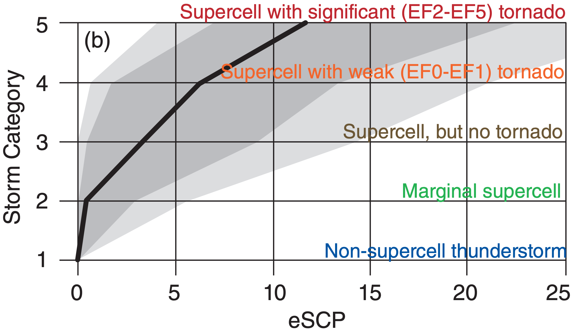
Because none of the forecast parameters and indices give perfect forecasts of supercells and tornadoes, researchers continue to develop and test other indices. One example is the effective Supercell Composite Parameter (eSCP), defined by:

\(\ \begin{align} \mathrm{eSCP}=\left(\mathrm{C} / \mathrm{C}_{o}\right) \cdot\left(\mathrm{H} / \mathrm{H}_{o}\right) \cdot\left(\mathrm{S} / \mathrm{S}_{0}\right)\tag{15.59}\end{align}\)

where C = MUCAPE, C_o = 1000 J kg^–1, H = eSRH, H_o = 50 m² s^–2, S = eBWD = effective bulk wind difference in the range of 10 to 20 m s^–1, and So = 20 m s^–1. eSCP is set to zero if S < 10 m s^–1. (S/S_o) is set to 1 if S > S_o. Fig. 15.50 shows how eSCP relates to right-moving supercells and tornadoes.

Another experimental parameter is the effective Significant Tornado Parameter (eSTP), which is defined only when the inflow base is at the ground:

\(\ \begin{align} \operatorname{eSTP}=\left(C / C_{1}\right) \cdot\left(\Delta L / L_{1}\right) \cdot\left(H / H_{1}\right) \cdot\left(S / S_{1}\right) \cdot\left(I+I_{1}\right) / I_{r}\tag{15.60}\end{align}\)

where C = MLCAPE, C₁ = 1500 J kg^–1, ∆L = [2000 m – L] for L = ML.LCL, L₁ = 1000 m, H = eSRH, H₁ = 150 m² s^–2, S = eBWD in the range of 12.5 to 30 m s^–1, S₁ = 20 m s^–1, I = ML.CIN, I₁ = 200 J kg^–1, and I_r = 150 J kg^–1. eSTP is set to zero if S < 12.5 m s^–1. (S/S₁) is set to 1.5 if S > 30 m s^–1. (∆L/L₁) is set to 1 for L < L₁. [(I+I₁)/I_r] is set to 1 for I > –50 J kg^–1. Fig. 15.51 shows how eSTP relates to supercells and tornadoes.

Figure 15.50 Statistics of thunderstorm intensity vs. effective Supercell Composite Parameter (eSCP). For several hundred right-moving storms in central N. America, the black line is the median (50 percentile); dark grey shading spans 25^th to 75^th percentiles (interquartile range); and light grey spans 10^th to 90^th percentiles.

Figure 15.51 Statistics of thunderstorm intensity vs. effective Significant Tornado Parameter (eSTP). For several hundred storms in central N. America, the black line is the median (50 percentile); dark grey shading spans 25^th to 75^th percentiles (the interquartile range); and light grey spans 10^th to 90^th percentiles.

15.4.9. Multiple-vortex Tornadoes

If conditions are right, a single parent tornado can develop multiple mini daughter-tornadoes around the parent-tornado perimeter near the ground (Fig. 15.52c). Each of these daughter vortices can have strong tangential winds and very low core pressure. These daughter tornadoes are also known as suction vortices or suction spots. Multiple-vortex tornadoes can have 2 to 6 suction vortices. The process of changing from a single vortex to multiple vortices is called tornado breakdown.

Figure 15.52 Sketch of the evolution of a tornado (blue shading) and how the bottom can separate into multiple vortices (red shading) as the swirl ratio (S) increases. The multiple suction vortices move around the perimeter (yellow arrow) of the parent tornado

A ratio called the swirl ratio can be used to anticipate tornado breakdown and the multi-vortex nature of a parent tornado:

\(\ \begin{align} S=M_{t a n} / W\tag{15.61}\end{align}\)

where W is the average updraft speed in a mesocyclone, and M_tan is the tangential wind component around the mesocyclone. If we idealize the mesocyclone as being cylindrical, then:

\(\ \begin{align} S=\frac{R_{M C} \cdot M_{t a n}}{2 z_{i} \cdot M_{r a d}}\tag{15.62}\end{align}\)

where M_rad is the inflow speed (i.e., radial velocity component,) R_MC is the radius of the mesocyclone, and z_i is the depth of the atmospheric boundary-layer. For the special case of R_MC ≈ 2·z_i , then:

\(\ \begin{align} S \approx M_{t a n} / M_{r a d}\tag{15.63}\end{align}\)

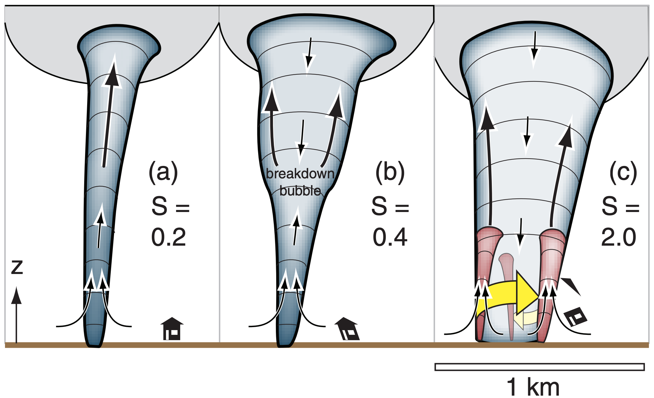
When the swirlratio is small (0.1 to 0.3), tornadoes have a single, well-defined, smooth-walled funnel (Fig. 15.52a), based on laboratory simulations. There is low pressure at the center of the tornado (tornado core), and the core contains updrafts at all heights. Core radius R_o of the tornado is typically 5% to 25% of the updraft radius, R_MC, in the mesocyclone.

If conditions change in the mesocyclone to have faster rotation and slower updraft, then the swirl ratio increases. This is accompanied by a turbulent downdraft in the top of the tornado core (Fig. 15.52b). The location where the core updraft and downdraft meet is called the breakdown bubble, and this stagnation point moves downward as the swirl ratio increases. The tornado is often wider above the stagnation point.

As the swirl ratio increases to a value of S* ≈ 0.45 (critical swirl ratio), the breakdown bubble gradually moves downward to the ground. The core now has a turbulent downdraft at all altitudes down to the ground, while around the core are strong turbulent updrafts around the larger-diameter tornado. At swirl ratios greater than the critical value, the parent tornado becomes a large-diameter helix of rotating turbulent updraft air, with a downdraft throughout the whole core.

At swirl ratios of about S ≥ 0.8, the parent tornado creates multiple daughter vortices around its perimeter (Fig 15.52c). As S continues to increase toward 3 and beyond, the number of multiple vortices increases from 2 up to 6.

Sample Application

At radius 2.5 km, a mesocyclone has a radial velocity of 1 m s^–1 and a tangential velocity of 3 m s^–1 . If the atmospheric boundary layer is 1.5 km thick, find the swirl ratio.

Find the Answer

Given: M_rad = 1 m s^–1, Mtan = 3 m s^–1, R_MC = 2500 m, and z_i = 1.5 km

Find: S = ? (dimensionless)

Although eq. (15.63) is easy to use, it contains some assumptions that might not hold for our situation. Instead, use eq. (15.62):

\(S=\frac{(2500 \mathrm{m}) \cdot(3 \mathrm{m} / \mathrm{s})}{2 \cdot(1500 \mathrm{m}) \cdot(1 \mathrm{m} / \mathrm{s})}=\underline{\mathbf{2.5}}\) (dimensionless)

Check: Physics and units OK.

Exposition: Because this swirl ratio exceeds the critical value, multiple vortices are likely.

Often W is not known and hard to measure. But using mass continuity, the vertical velocity in eq. (15.61) can be estimated from the radial velocity for eq. (15.62), which can be easier to estimate.

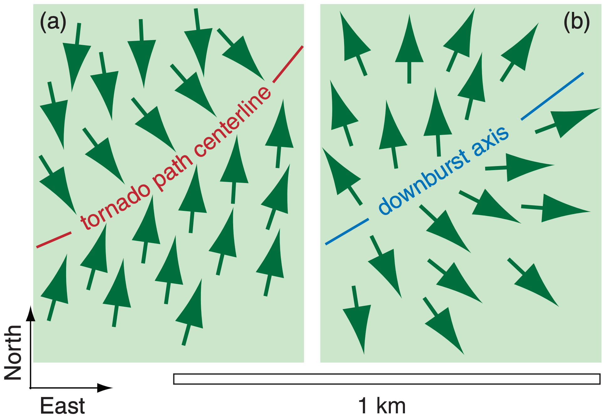
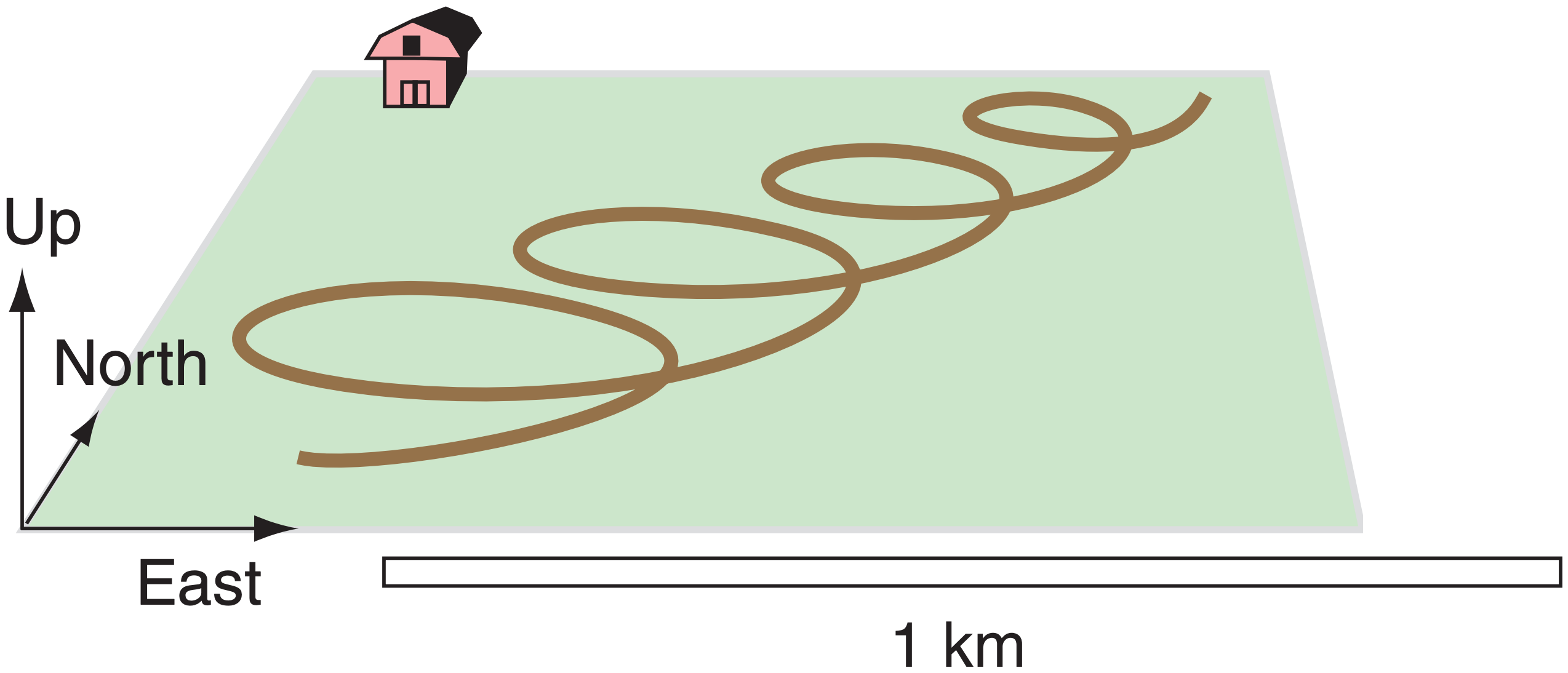
Wind speeds and damage are greatest in these small suction vortices. The individual vortices not only circulate around the perimeter of the parent tornado, but the whole tornado system translates over the ground as the thunderstorm moves across the land. Thus, each vortex traces a cycloidal pattern on the ground, which is evident in post-tornado aerial photographs as cycloidal damage paths to crops (Fig. 15.53).

Figure 15.53 Cycloidal damage path in a farm field caused by a tornadic suction vortex embedded in a larger diameter parent tornado.

When single-vortex tornadoes move over a forest, they blow down the trees in a unique pattern that differs from tree blowdown patterns caused by straight-line downburst winds (Fig. 15.54). Sometimes these patterns are apparent only from an aerial vantage point.

Figure 15.54 Damage signatures of (a) tornadoes and (b) downbursts in a forest, as seen in aerial photographs of tree blowdown. Green arrows represent blown-down trees.