12.2: Airmasses

An airmass is a widespread (of order 1000 km wide) body of air in the bottom third of the troposphere that has somewhat-uniform characteristics. These characteristics can include one or more of: temperature, humidity, visibility, odor, pollen concentration, dust concentration, pollutant concentration, radioactivity, cloud condensation nuclei (CCN) activity, cloudiness, static stability, and turbulence.

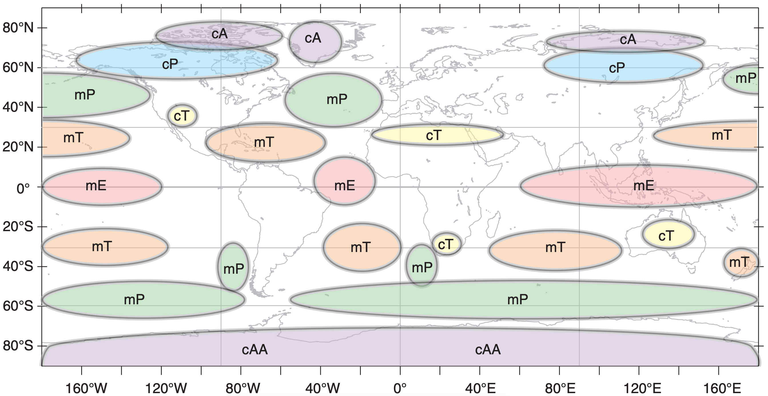
Airmasses are usually classified by their temperature and humidity, as associated with their source regions. These are usually abbreviated with a twoletter code. The first letter, in lowercase, describes the humidity source. The second letter, in uppercase, describes the temperature source. Table 12-1 shows airmass codes. [CAUTION: In Great Britain, the two letters are reversed.]

Examples are maritime Tropical (mT) airmasses, such as can form over the Gulf of Mexico, and continental Polar (cP) air, such as can form in winter over Canada.

After the weather pattern changes and the airmass is blown away from its genesis region, it flows over surfaces with different relative temperatures. Some organizations append a third letter to the end of the airmass code, indicating whether the moving airmass is (w) warmer or (k) colder than the underlying surface. This coding helps indicate the likely static stability of the air and the associated weather. For example, “mPk” is humid cold air moving over warmer ground, which would likely be statically unstable and have convective clouds and showers.

Table 12-1. Airmass abbreviations. Boldface indicates the most common ones.
Abbr.	Name	Description
c	continental	Dry. Formed over land.
m	maritime	Humid. Formed over ocean.
A	Arctic	Very cold. Formed in the polar high.
E	Equatorial	Hot. Formed near equator
M	Monsoon	Similar to tropical.
P	Polar	Cold. Formed in subpolar area.
S	Superior	A warm dry airmass having its origin aloft.
T	Tropical	Warm. Formed in the subtropical high belt.
k	colder than the underlying surface
w	warmer than the underlying surface
Special (regional) abbreviations.
AA	Antarctic	Exceptionally cold and dry.
r	returning	As in “rPm” returning Polar maritime [Great Britain].
Note: Layered airmasses are written like a fraction, with the airmass aloft written above a horizontal line and the surface airmass written below. For example, just east of a dryline you might have: \(\frac{\mathrm{cT}}{\mathrm{mT}}\)

Sample Application

A “cA“ airmass has what characteristics?

Find the Answer

Given: cA airmass.

Find: characteristics

Use Table 12-1: cA = continental Arctic

Characteristics: Dry and very cold.

Check: Agrees with Fig. 12.4.

Exposition: Forms over land in the arctic, under the polar high. In Great Britain, the same airmass is labeled as Ac.

12.2.1. Creation

An airmass can form when air remains stagnant over a surface for sufficient duration to take on characteristics similar to that surface. Also, an airmass can form in moving air if the surface over which it moves has uniform characteristics over a large area. Surface high-pressure centers favor the formation of airmasses because the calm or light winds allow long residence times. Thus, many of the airmass genesis (formation) regions (Fig. 12.4) correspond to the planetary- and continental-scale high-pressure regions described in the previous section.

Figure 12.4 Airmass formation regions (symbols are defined in Table 12-1). Some meteorologists change all “mE” to “mT”, and “cAA” to “cA”.

Airmasses form as boundary layers. During their residence over a surface, the air is modified by processes including radiation, conduction, divergence, and turbulent transport between the ground and the air.

12.2.1.1. Warm Airmass Genesis

When cool air moves over a warmer surface, the warm surface modifies the bottom of the air to create an evolving, convective mixed layer (ML). Turbulence — driven by the potential temperature difference ∆θ_s between the warm surface θ_sfc and the cooler airmass θ_ML — causes the ML depth z_i to initially increase (Fig. 12.5). This is the depth of the new airmass. A heat flux from the warm surface into the air causes θ_ML to warm toward θ_sfc. θ_ML is the temperature of the new airmass as it warms.

Figure 12.5 Genesis of a warm airmass after cold air comes to rest over a warmer surface. This is an example based on toy-model equations in the INFO Box. Airmass potential temperature is θ_ML and depth is z_i . Imposed conditions for this case-study example are: large-scale divergence β = 10^–6 s^–1, potential temperature gradient in vertical γ_o = 3.3 K km^–1, initial near-surface air potential temperature θ_ML = θ_o = 10°C, and surface temperature θ_sfc = 20°C.

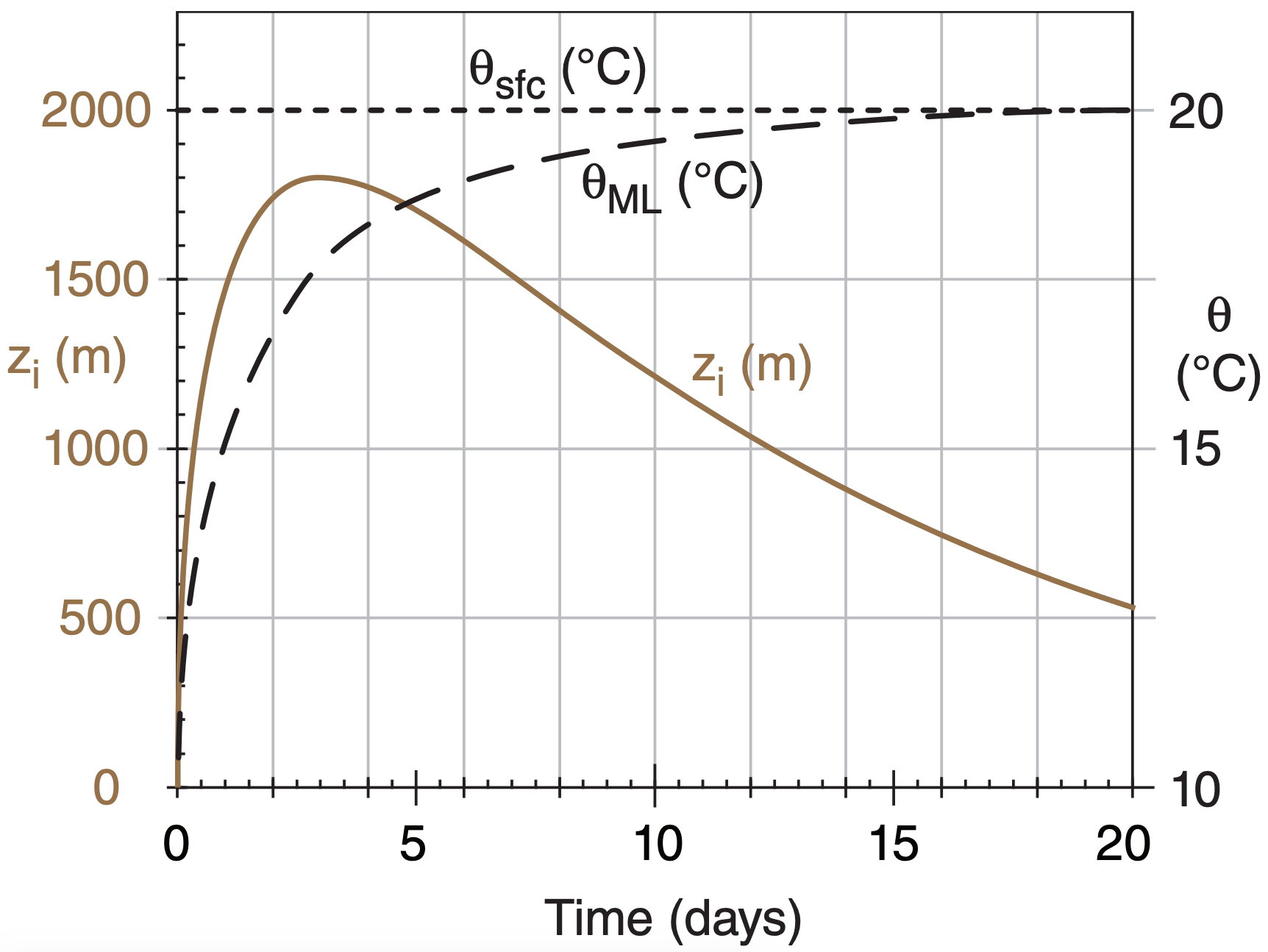
Synoptic-scale divergence β and subsidence ws, which is expected in high-pressure airmass-genesis regions, oppose the ML growth. Changes within the new airmass are rapid at first. But as airmass temperature gradually approaches surface temperature, the turbulence diminishes and so does the rate of ML depth increase. Eventually, the ML depth begins to decrease (Fig. 12.5) because the reduced turbulence (trying to increase the ML thickness) cannot counteract the relentless subsidence.

A “toy model” describing the atmospheric boundary-layer processes that create a warm airmass is given in the INFO Box. The nearby Sample Application box uses this toy model to find the evolution of the warm airmass depth (i.e., the ML depth z_i ) and its potential temperature θ_ML evolution. This is the solution that was plotted in Fig. 12.5.

The e-folding time (see Chapter 1) for the θ_ML to approach θ_sfc is surprisingly constant — about 1 to 2 days. As a result, creation of this warm tropical airmass is nearly complete after about a week. That is how long it takes until the airmass temperature nearly equals the surface temperature (Fig. 12.5). The time \(\ \tau\) to reach the peak ML thickness is typically about 1 to 4 days (see another INFO box).

A SCIENTIFIC PERSPECTIVE • Math Clarity

In math classes, you might have learned how to combine many small equations into a single large equation that you can solve. For meteorology, although we could make such large single-equation combinations, we usually cannot solve them.

So there is no point in combining all the equations. Instead, it is easier to see the physics involved by keeping separate equations for each physical process. An example is the toy model given in the INFO Box on the next page for warm airmass genesis. Even though the many equations are coupled, it is clearer to keep them separate.

INFO • Bergen School of Meteorology

During World War I, Vilhelm Bjerknes, a Norwegian physicist with expertise in radio science and fluid mechanics, was asked in 1918 to form a Geophysical Institute in Bergen, Norway. Cut-off from weather data due to the war, he arranged for a dense network of 60 surface weather stations to be installed. Some of his students were C.-G. Rossby, H. Solberg, T. Bergeron, V. W. Ekman, H. U. Sverdrup, and his son Jacob Bjerknes.

Jacob Bjerknes used the weather station data to identify and classify cold, warm, and occluded fronts. He published his results in 1919, at age 22. The term “front” supposedly came by analogy to the battle fronts during the war. He and Solberg also later explained the life cycle of cyclones. Their description is known as the Norwegian cyclone model.

INFO • Warm Airmass Genesis

Modeling warm airmass creation (genesis) is an exercise in atmospheric boundary-layer (ABL) evolution. Since we do not cover ABLs in detail until a later chapter, the details are relegated to this INFO Box. You can safely skip them now, and come back later after you have studied ABLs.

Define a relative potential temperature θ based on a reference height (z) at the surface (z = 0). Namely, θ ≈ T + Γ_d · z, where Γ_d = 9.8 °C km^–1 is the dry adiabatic lapse rate.

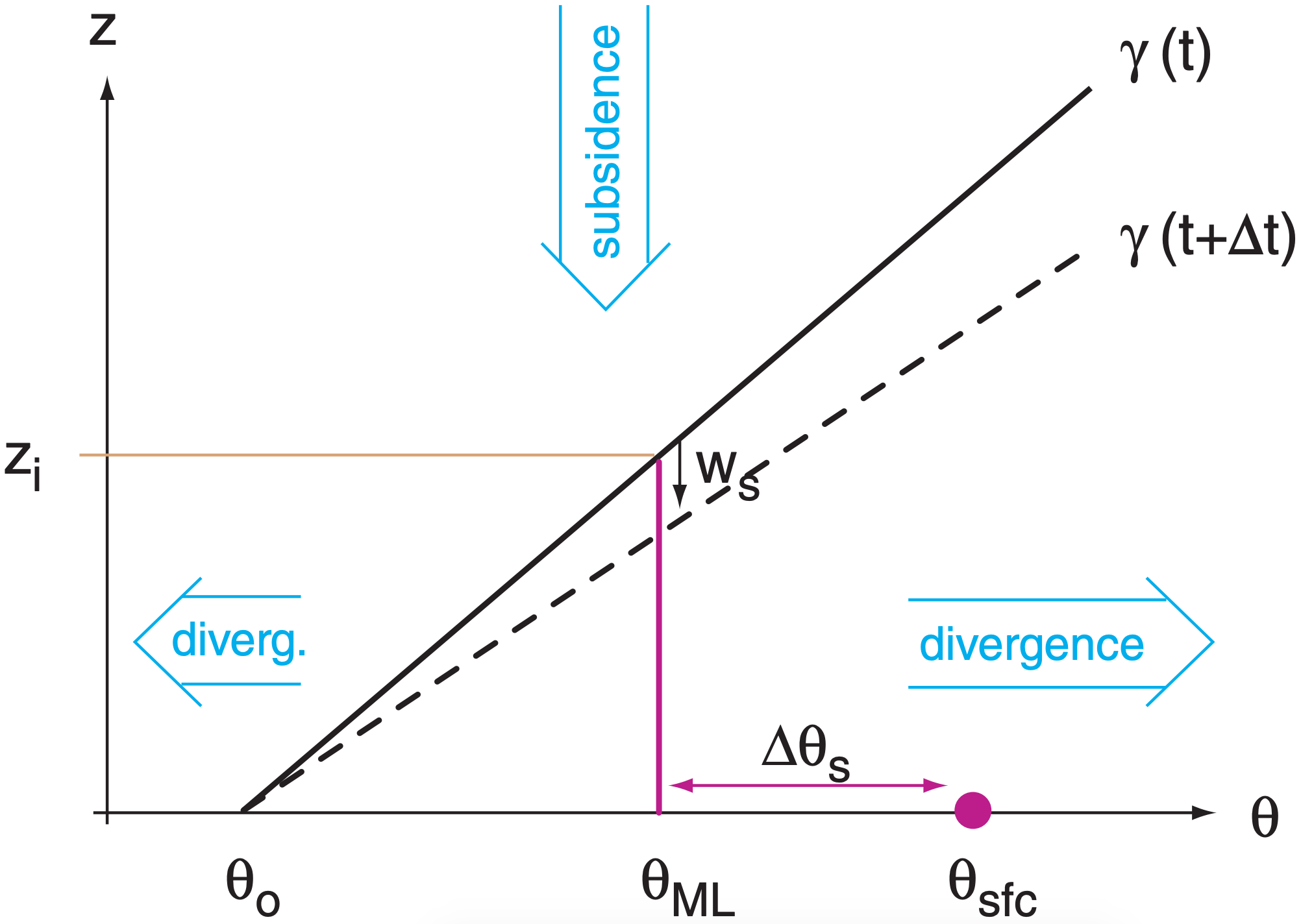
Suppose that a cool, statically stable layer of air initially (subscript o) has a near-surface temperature of θ_o and a linear potential-temperature gradient γ_o = γ = ∆θ/∆z before it comes to rest over a warm surface of temperature θ_sfc (see Fig. above). We want to predict the time evolution of the depth (z_i ) and potential temperature (θ_ML) of this new airmass. Because this airmass is an ABL, we can use boundary-layer equations to predict z_i (the height of the convective mixed-layer ,ML), and θ_ML (the ML potential temperature).

ML depth increases by amount ∆z_ie during a time interval ∆t due to thermodynamic encroachment (i.e., warming under the capping sounding). This is an entrainment process that adds air to the ML through the ML top. Large scale divergence β = ∆ / U x ∆ ∆ + V y / ∆ removes air horizontally from the ML and causes a subsidence velocity of magnitude w_s at the ML top:

\(\ \begin{align} w_{s}=\beta \cdot z_{i}^{*}\tag{7}\end{align}\)

Thus, a change in ML depth results from the competition of these two terms:

\(\ \begin{align} z_{i}=z_{i}^{*}+\Delta z_{i e}-w_{s} \cdot \Delta t\tag{12}\end{align}\)

where the asterisk * indicates a value from the previous time step.

The amount of heat ∆Q (as an incremental accumulated kinematic heat flux) transferred from the warm surface to the cooler air during time interval ∆t under light-wind conditions depends on the temperature difference at the surface ∆θ_s and the intensity of turbulence, as quantified by a buoyancy velocity scale w_b:

\(\ \begin{align} \Delta Q=b \cdot w_{b} \cdot \Delta \theta_{s} \cdot \Delta t\tag{10}\end{align}\)

where b = 5x10^–4 (dimensionless) is a convective heat transport coefficient (see the Heat chapter).

The buoyancy velocity scale is:

\(\ \begin{align} w_{b}=\left[\frac{|g|}{\theta_{M L}^{*}} \cdot z_{i}^{*} \cdot \Delta \theta_{s}\right]^{1 / 2}\tag{9}\end{align}\)

where |g| = 9.8 m s^–2 is gravitational acceleration.

That heat goes to warming θ_ML, which by geometry adds a trapezoidal area under the γ curve :

\(\ \begin{align} \Delta z_{i e}=\left[\frac{2 \cdot \Delta Q}{\gamma}+\left(z_{i}^{*}\right)^{2}\right]^{1 / 2}-z_{i}^{*}\tag{11}\end{align}\)

Knowing the entrainment rate, we get ∆θ_ML geometrically from where it intercepts the γ curve:

\(\ \begin{align} \theta_{M L}=\theta_{M L}^{*}+\gamma \cdot \Delta z_{i e}\tag{13}\end{align}\)

With this new ML temperature, we can update the surface temperature difference

\(\ \begin{align} \Delta \theta_{s}=\theta_{s f c}-\theta_{M L}^{*}\tag{8}\end{align}\)

Knowing the large-scale divergence, we can also update the potential temperature profile in the air above the ML:

\(\ \begin{align} \gamma=\gamma_{o} \cdot \exp (\beta \cdot t)\tag{6}\end{align}\)

All that remains is to update the time variable:

\(\ \begin{align} t=t^{*}+\Delta t\tag{5}\end{align}\)

You might have noticed that some of the equations above are initially singular, when the ML has zero depth. So, for the first small time step (∆t ≈ 6 minutes = 360 s), you should use the following special equations in the following order:

\(\ \begin{align} t=\Delta t\tag{1}\end{align}\)

\(\ \begin{align} \Delta \theta_{S}=\theta_{s f c}-\theta_{o}\tag{2}\end{align}\)

\(\ \begin{align} z_{i}=\Delta \theta_{s} \cdot\left[\frac{2 \cdot b \cdot \Delta t}{\gamma_{o}} \cdot\left(\frac{|g|}{\theta_{o}}\right)^{1 / 2}\right]^{2 / 3}\tag{3}\end{align}\)

\(\ \begin{align} \theta_{M L}=\theta_{o}+\gamma_{o} \cdot z_{i}\tag{4}\end{align}\)

Then, for all the subsequent time steps, use the set of equations (5 to 13 in the order as numbered) to find the resulting ML evolution. Repeat eqs. (5 to 13) for each subsequent step. As the solution begins to change more gradually, you may use larger time steps ∆t. The result is a toy model that describes warm airmass formation as an evolving convective boundary layer.

The Sample Application on the next page shows how this can be done with a computer spreadsheet. First, you need to specify the imposed constants γ_o , θ_o, β and θ_sfc. Next, initialize the values of: γ = γ_o , z_i = 0, and θ_ML = θ_o at t = 0 . Then, solve the equations for the first step. Finally, continue iterating for subsequent time steps to simulate warm airmass genesis.

These simulations show that greater divergence causes a shallower ML that can warm faster. Greater static stability in the ambient environment reduces the peak ML depth.

Sample Application (§)

Air of initial ML potential temperature 10°C comes to rest over a 20°C sea surface. Divergence is 10^–6 s^–1, and the initial ∆θ/∆z = γ = 3.3 K km^–1. Find and plot the warm airmass evolution of potential temperature and depth.

Find the Answer

Given: θ_o = 10°C = 283K, θ_sfc = 20°C, γ_o = 3.3 K km^–1, β = 10^–6 s^–1.

Find: θ_ML(t) = ? °C, z_i (t) = ? m

For the first time step of ∆t = 6 min (=360 s), use eqs. (1 to 4 from the INFO Box on the previous page). For subsequent steps, repeatedly use eqs. (5 to 13 from that same INFO Box).

t (s)	t (d)	γ (K m^–1)	ws (m s^–1)	∆θs (°C)	wb (m s^–1)	∆Q (K·m)	∆zie (m)	zi (m)	θML (°C)
0	0.000							0	10
360	0.004			10				74	10.2
720	0.008	0.00330	0.00007	9.75	5.0	8.8	29.8	104	10.3
1080	0.013	0.00330	0.00010	9.66	5.9	10.3	26.4	131	10.4
1440	0.017	0.00330	0.00013	9.57	6.6	11.3	24.0	155	10.5
. . .
259200	3.00	0.00428	0.00179	2.41	12.0	104.3	13.6	1789	17.7
270000	3.13	0.00432	0.00179	2.35	11.9	150.8	19.4	1789	17.7
280800	3.25	0.00437	0.00179	2.26	11.7	142.8	18.2	1788	17.8
. . .
1684800	19.50	0.01779	0.00057	0.14	1.6	4.9	0.5	542	19.9
1728000	20.00	0.01858	0.00054	0.13	1.5	4.4	0.4	519	19.9

Sample results from the computer spreadsheet are shown above. The final answer is plotted in Fig. 12.5.

Check: Units OK. Physics OK. Fig. 12.5 reasonable.

Exposition: I used small time steps of ∆t = 6 minutes initially, and then as ∆z_ie became smaller, I gradually increased past ∆t = 3 h to ∆t = 12 h. The figure shows rapid initial modification of the cold, statically stable airmass toward a warm, unstable airmass. Maximum z_i is reached in about \(\ \tau\) = 3.06 days (see INFO box), in agreement with Fig. 12.5.

INFO • Time of Max Airmass Thickness

The time \(\ \tau\) to reach the peak ML thickness for warm airmass genesis is roughly

\(\ \begin{align} \tau \approx c \cdot\left(\frac{\theta_{0}}{|g| \cdot \beta \cdot \gamma_{o} \cdot e^{\beta \cdot \tau}}\right)^{1 / 3}\tag{c}\end{align}\)

where c = 140 (dimensionless), and the other variables are defined in the text. \(\ \tau\) is typically about 1 to 4 days. Any further lingering of the airmass over the same surface temperature results in a loss of airmass thickness due to divergence.

Equation (c) is an implicit equation; namely, you need to know \(\ \tau\) in order to solve for \(\ \tau\). Although this equation is difficult to solve analytically, you can iterate to quickly converge to a solution in about 5 steps in a computer spreadsheet. Namely, start with \(\ \tau\) = 0 as the first guess and plug into the right side of eq. (c). Then solve for \(\ \tau\) on the left side. For the next iteration, take this new \(\ \tau\) and plug it in on the right, and solve for an updated \(\ \tau\) on the left. Repeat until the value of \(\ \tau\) converges to a solution; namely, when ∆\(\ \tau\)/\(\ \tau\) < ε for ε = 0.01 or smaller.

Sample Application (§)

For the conditions of the previous Sample Application, find the time \(\ \tau\) that estimates when the new warm airmass has maximum thickness.

Find the Answer

Given: θ_o = 10°C = 283K, θ_sfc = 20°C, γ_o = 3.3 K km^–1, β = 10^–6 s^–1.

Find: \(\ \tau\) = ? days

Use eq. (c) from the INFO Box at left. Start with \(\ \tau\) = 0. The first iteration is:

\(\tau=140 \cdot\left[\frac{283 \mathrm{K}}{\left(9.8 \mathrm{m} / \mathrm{s}^{2}\right) \cdot\left(10^{-6} \mathrm{s}^{-1}\right) \cdot(0.0033 \mathrm{K} / \mathrm{m}) \cdot e^{0}}\right]^{1 / 3}\)

= 288498 s = 3.339 days

Subsequent iterations give: \(\tau=\)

3.033 -> 3.060 -> 3.057 -> 3.058 -> 3.058 days

Check: Units OK. Physics OK. Agrees with Fig. 12.5.

Exposition: Convergence was quick. From Fig. 12.5, the actual time of this peak thickness was between 3 and 3.125 days, so eq. (c) does a reasonable job.

12.2.1.2. Cold Airmass Genesis

When air moves over a colder surface such as arctic ice, the bottom of the air first cools by conduction, radiation, and turbulent transfer with the ground. Turbulence intensity then decreases within the increasingly statically-stable boundary layer, reducing the turbulent heat transport to the cold surface.

However, direct radiative cooling of the air, both upward to space and downward to the cold ice surface, chills the air at a rate of 2°C day^–1 (averaged over a 1 km thick boundary layer). As the air cools below the dew point, water-droplet clouds form. Continued radiative cooling from cloud top allows ice crystals to grow at the expense of evaporating liquid droplets, changing the cloud into an ice cloud.

Radiative cooling from cloud top creates cloudy “thermals” of cold air that sink, causing some turbulence that distributes the cooling over a deeper layer. Turbulent entrainment of air from above cloud top down into the cloud allows the cloud top to rise, and deepens the incipient airmass (Fig. 12.6).

Figure 12.6 Genesis of a continental-polar air mass over arctic ice. The cloud/fog regions are shaded in light blue.

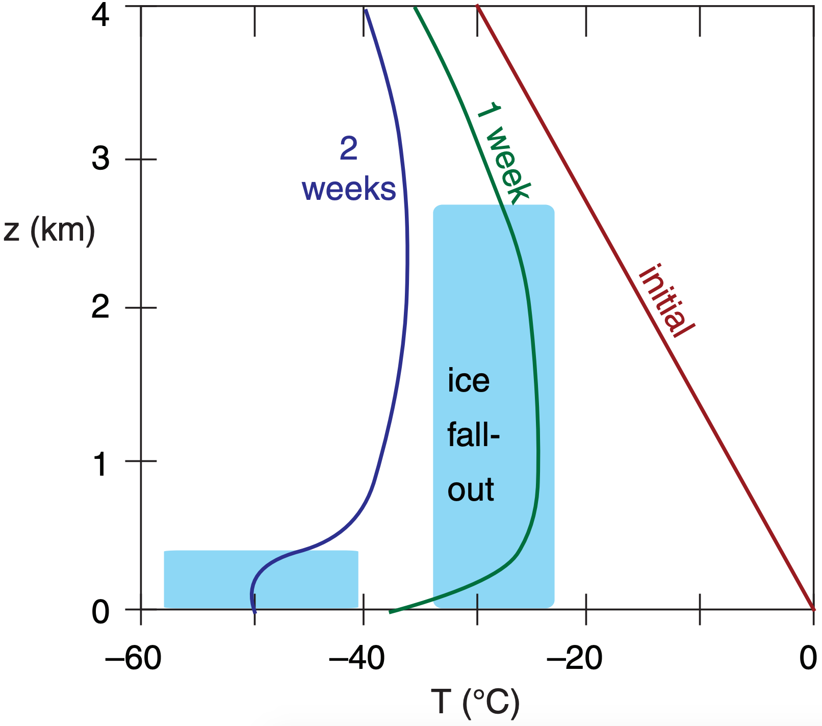
The ice crystals within this cloud are so few and far between that the weather is described as cloudless ice-crystal precipitation. This can create some spectacular halos and other optical phenomena in sunlight (see the Atmospheric Optics chapter), including sparkling ice crystals known as diamond dust. Nevertheless, infrared radiative cooling in this cloudy air is much greater than in clear air, allowing the cooling rate to increase to 3°C day–1 over a layer as deep as 4 km.

During the two-week formation of this continental-polar or continental-arctic airmass, most of the ice crystals precipitate out leaving a thinner cloud of 1 km depth. Also, subsidence within the high pressure reduces the thickness of the cloudy airmass and causes some warming to partially counteract the radiative cooling.

Above the final fog layer is a nearly isothermal layer of air 3 to 4 km thick that has cooled about 30°C. Final air-mass temperatures are often in the range of –30 to –50 °C, with even colder temperatures near the surface.

While the Arctic surface consists of relatively flat sea-ice (except for Greenland), the Antarctic has mountains, high ice-fields, and significant surface topography (Fig. 12.7). As cold air forms by radiation, it can drain downslope as a katabatic wind (see the Regional Winds chapter). Steady winds of 10 m s^–1 are common in the Antarctic interior, with speeds of 50 m s^–1 along some of the steeper slopes.

Figure 12.7 Cold katabatic winds (dark-blue arrow) draining from Antarctica.

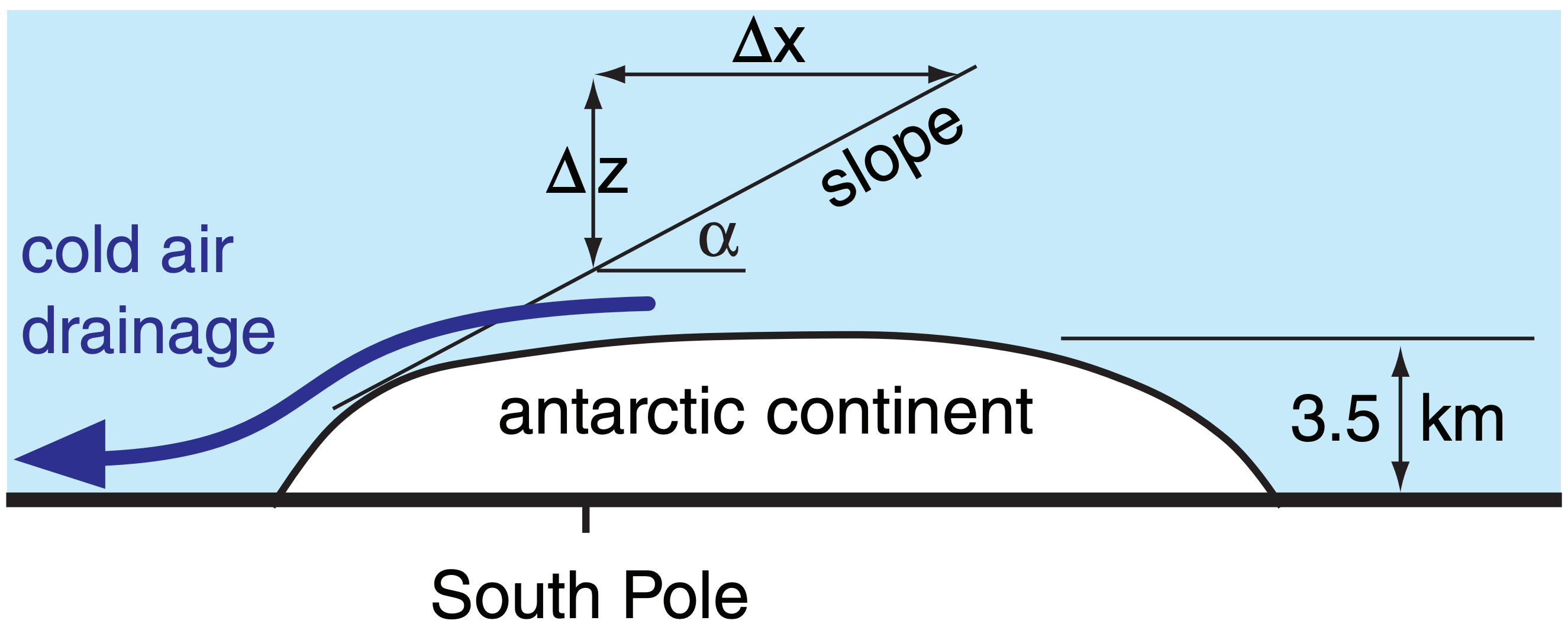
As will be shown in the Regional Winds chapter, the buoyancy force per unit mass on a surface of slope ∆z/∆x translates into a quasi-horizontal slopeforce per mass of:

\( \begin{align} \frac{F_{x S}}{m}=\frac{|g| \cdot \Delta \theta}{T_{e}} \cdot \frac{\Delta z}{\Delta x}\tag{12.1}\end{align}\)

\(\ \begin{align} \frac{F_{y S}}{m}=\frac{|g| \cdot \Delta \theta}{T_{e}} \cdot \frac{\Delta z}{\Delta y}\tag{12.2}\end{align}\)

where |g| = 9.8 m·s^–2 is gravitational acceleration, and ∆θ is the potential-temperature difference between the draining cold air and the ambient air above. The ambient-air absolute temperature is T_e.

Sample Application

Find the slope force per unit area acting on a katabatic wind of temperature –20°C with ambient air temperature 0°C. Assume a slope of ∆z/∆x = 0.1 .

Find the Answer

Given: ∆θ = 20 K, T_e = 273 K, ∆z/∆x = 0.1

Find: F_{x S}/m = ? m·s^–2

Use eq. (12.1):

\(\frac{F_{x} s}{m}=\frac{\left(9.8 \mathrm{m} \cdot \mathrm{s}^{-2}\right) \cdot(20 \mathrm{K})}{273 \mathrm{K}} \cdot(0.1)\)

= 0.072 m·s^–2

Check: Units OK. Physics OK.

Exposition: This is two orders of magnitude greater than the typical synoptic forces (see the Dynamics chapter). Hence, drainage winds can be strong.

The sign of these forces should be such as to accelerate the wind downslope. The equations above work when the magnitude of slope ∆z/∆x is small, because then ∆z/∆x = sin(α), where α is the slope angle of the topography.

The katabatic wind speed in the Antarctic also depends on turbulent drag force against the ice surface, ambient pressure-gradient force associated with synoptic weather systems, Coriolis force, and turbulent drag caused by mixing of the draining air with the stationary air above it. At an average drainage velocity of 5 m s^–1, air would need over 2 days to move from the interior to the periphery of the continent, which is a time scale on the same order as the inverse of the Coriolis parameter. Hence, Coriolis force cannot be neglected.

Katabatic drainage removes cold air from the genesis regions and causes turbulent mixing of the cold air with warmer air aloft. The resulting coldair mixture is rapidly distributed toward the outside edges of the antarctic continent.

One aspect of the global circulation is a wind that blows around the poles. This is called the polar vortex. Katabatic removal of air from over the antarctic reduces the troposphere depth, enhancing the persistence and strength of the antarctic polar vortex due to potential vorticity conservation.

12.2.2. Movement

Airmasses do not remain stationary over their birth place forever. After a week or two, a transient change in the weather pattern can push the airmass toward new locations.

When airmasses move, two things can happen: (1) As the air moves over surfaces with different characteristics, the airmass begins to change. This is called airmass modification, and is described in the next subsection.

(2) An airmass can encounter another airmass. The boundary between these two airmasses is called a front, and is a location of strong gradients of temperature, humidity, and other airmass characteristics. Fronts are described in detail later.

Tall mountain ranges can strongly block or channel the movement of airmasses, because airmasses occupy the bottom of the troposphere. Fig. 12.8 shows a simplified geography of major mountain ranges.

Figure 12.8 Locations of major mountain ranges (brown lines), lesser ranges (tan lines), and large plateaus of land or ice (tan ovals).

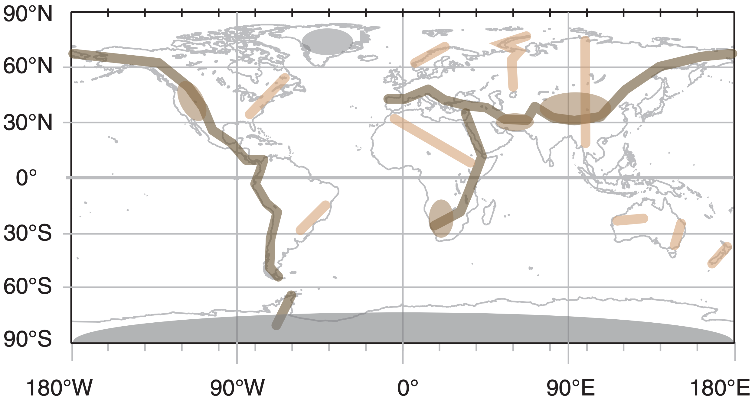
For example, in the middle of North America, the lack of any major east-west mountain range allows the easy movement of cold polar air from Canada toward warm humid air from the Gulf of Mexico. This sets the stage for strong storms (see the Extratropical Cyclone chapter and the chapters on Thunderstorms).

The long north-south barrier of mountains (Rockies, Sierra Nevada, Cascades, Coast Range) along the west coast of North America impedes the easy entry of Pacific airmasses toward the center of that continent. Those mountains also help protect the west coast from the temperature extremes experienced by the rest of the continent.

In Europe, the mountain orientation is the opposite. The Alps and the Pyrenees are east-west mountain ranges that inhibit movement of Mediterranean airmasses from reaching northward. The lack of major north-south ranges in west and central Europe allows the easy movement of maritime airmasses from the Atlantic to sweep eastward, bringing cool wet conditions.

One of the greatest ranges is the Himalaya Mountains, running east-west between India and China. Maritime tropical airmasses moving in from the Indian Ocean reach these mountains, causing heavy rains over India during the monsoon. The same mountains block the maritime air from reaching further northward, leaving a very dry Tibetan Plateau and Gobi Desert in its rain shadow.

The discussion above focused on blocking and channeling by the mountains. In some situations air can move over mountain tops (Fig. 12.9). When this happens, the airmass is strongly modified, as described next.

12.2.3. Modification

As an airmass moves from its origin, it is modified by the new landscapes under it. For example, a polar airmass will warm and gain moisture as it moves equatorward over warmer vegetated ground. Thus, it gradually loses its original identity.

12.2.3.1. Via Surface Fluxes

Heat and moisture transfer at the surface can be described with bulk-transfer relationships such as eq. (3.34). If we assume for simplicity that wind-induced turbulence creates a well-mixed airmass of quasi-constant thickness z_i , then the change of airmass potential temperature θML with travel-distance ∆x is:

\(\ \begin{align} \frac{\Delta \theta_{M L}}{\Delta x} \approx \frac{C_{H} \cdot\left(\theta_{s f c}-\theta_{M L}\right)}{z_{i}}\tag{12.3}\end{align}\)

where C_H ≈ 0.01 is the bulk-transfer coefficient for heat (see the chapters on Heat and on the Atmospheric Boundary Layer).

If the surface temperature is horizontally homogeneous, then eq. (12.3) can be solved for the airmass temperature at any distance x from its origin:

\(\ \begin{align} \theta_{M L}=\theta_{s f c}-\left(\theta_{s f c}-\theta_{M L\ o} \right) \cdot \exp \left(-\frac{C_{H} \cdot x}{z_{i}}\right)\tag{12.4}\end{align}\)

where θ_{ML o} is the initial airmass potential temperature at location x = 0.

Figure 12.9 Modification of a Pacific airmass by flow over mountains in the northwestern USA. (Numbers are used in the Sample Application.)

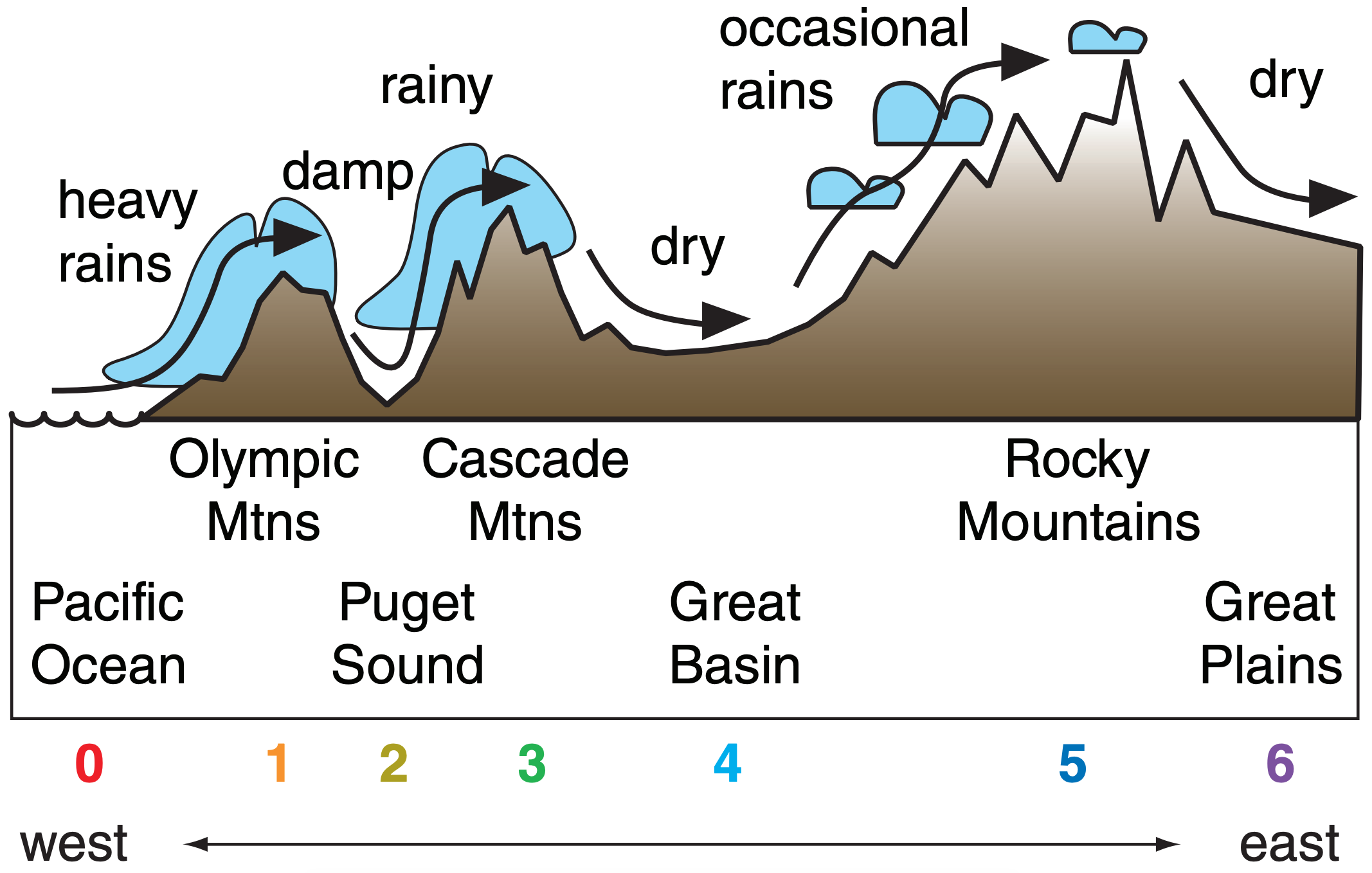
Sample Application

An mP airmass initially has T = 5°C & RH = 100%. Use a thermo diagram to find T & RH at: 1 Olympic Mtns. (elevation ≈ 1000 m), 2 Puget Sound (0 m), 3 Cascade Mtns (1500 m), 4 the Great Basin (500 m), 5 Rocky Mtns (2000 m), 6 the western Great Plains (1000 m)

Find the Answer

Given: Elevations from west to east (m) = 0, 1000, 0, 1500, 500, 2000, 1000 Initially RH=100%. Thus T_d = T = 5°C

Find: T (°C) & RH (%) at surface locations 1 to 6.

Assume: All condensation precipitates out. No additional heat or moisture transfer from the surface.

Start with air near sea level, where P_SL = 100 kPa.

Use Fig. 12.9 and an emagram from the Stability chapter. On the thermo diagram, the air parcel follows the following route: 0 - 1 - 2 - 1 - 3 - 4 - 3 - 5 - 6.

Initially (point 0), T_d = T = 5°C. Because this air is already saturated, it would follow a saturated adiabat from point 0 to point 1 at z = 1 km, where the still-saturated air has T_d = T = –1°C.

If all condensates precipitate out, then air would descend dry adiabatically (with T_d following an isohume) from point 1 to 2, giving T = 9°C and T_d = 1°C.

When this unsaturated air rises, it first does so dry adiabatically until it reaches its LCL at point 1. This now-cloudy air continues to rise toward point 3 moist adiabatically, where it has T_d = T = –4°C. Etc.

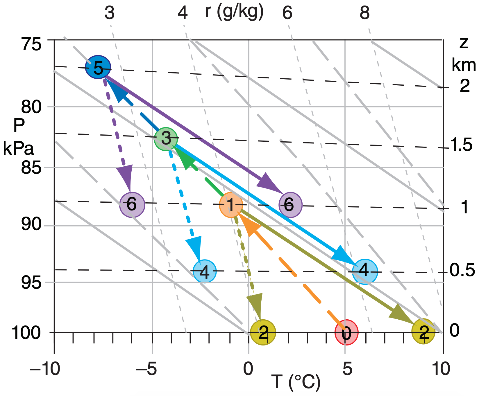
Results, where Index = circled numbers in Fig above.

Index	z (km)	T (°C)	Td (°C)	RH (%)
0	0	5	5	100
1	1	–1	–1	100
2	0	9	1	55
3	1.5	–4	–4	100
4	0.5	6	–2	54
5	2	–7	–7	100
6	1	2	–6	53

Check: Units OK. Physics OK. Figure OK.

Exposition: The airmass has lost its maritime identity by the time it reaches the Great Plains, and little moisture remains. Humidity for rain in the plains comes from the southeast (not from the Pacific).

Sample Application

A polar airmass with initial θ = –20°C and depth = 500 m moves southward over a surface of 0°C. Find the initial rate of temperature change with distance.

Find the Answer

Given: θ_ML = –20°C, θ_sfc = 0°C, z_i = 500 m

Find: ∆θ_ML /∆x = ? °C km–1. Assume no mountains.

Use eq. (12.3):

\(\frac{\Delta \theta_{M L}}{\Delta x} \approx \frac{(0.01) \cdot\left[0^{\circ} \mathrm{C}-\left(-20^{\circ} \mathrm{C}\right)\right]}{(500 \mathrm{m})}=\underline{0.4}^{\circ} \mathrm{C}\ \mathrm{km}^{-1}\)

Check: Units OK. Physics OK.

Exposition: Neither this answer nor eq. (12.4) depend on wind speed. While faster speeds give faster position change, they also cause greater heat transfer to/ from the surface (eq. 3.34). These 2 effects cancel.

12.2.3.2. Via Flow Over Mountains

If an airmass is forced to rise over mountain ranges, the resulting condensation, precipitation, and latent heating will dry and warm the air. For example, an airmass over the Pacific Ocean near the northwestern USA is often classified as maritime polar (mP), because it is relatively cool and humid. As the prevailing westerly winds move this airmass over the Olympic Mountains (a coastal mountain range), the Cascade Mountains, and the Rocky Mountains, there is substantial precipitation and latent heating (Fig. 12.9).