8.4: Homework Exercises

8.5.1. Broaden Knowledge & Comprehension

B1. Search the web for graphs of transmittance for wavelengths greater than 100 cm (like Figs. 8.4), and find the names of these regions of the electromagnetic spectrum. Comment on the possibility for remote sensing at these longer wavelengths.

B2. Search the web for graphs of weighting functions for one of the newer weather satellites, as specified by your instructor. Discuss their advantages and disadvantages compared to the weighting functions given in this book.

B3. Search the web for current orbital characteristics for the active weather satellite(s) specified by your instructor. Also, look for photos or artist drawings of these satellites.

B4. Search the web for data to create tables that list the names and locations (longitude for GOES; equator crossing times for POES) currently active weather satellites around the world. Discuss any gaps in worldwide weather-satellite coverage.

B5. Search the web for images from all the different channels for one of the satellites, as specified by your instructor. Discuss the value and utility of each image.

B6. Search the web for satellite loops that cover your location. Compare these images with the weather you see out the window, and make a short-term forecast based on the satellite loop.

B7. Search the web to find the most recent set of visible, IR, and water-vapor images that covers your area. Print these images; label cloud areas as (a), (b), etc.; and interpret the clouds in those images. For the cloud area directly over you, compare you satellite interpretation with the view out your window.

B8. Search the web for thermo diagrams showing temperature soundings as retrieved from satellite sounder radiance data. Compare one of these soundings with the nearest rawinsonde (in-situ) sounding (by searching on “upper air” soundings).

B9. Search the web for tutorials on satellite-image interpretation; learn how to better interpret one type of cloud system (e.g., lows, fronts, thunderstorms); and write a summary tutorial for your classmates.

B10. Search the web for galleries of classical satellite images showing the best examples of different types of clouds systems (e.g., hurricanes, squall lines).

B11. Compare high-resolution satellite images from Earth-observing satellites (Aqua, Terra, and newer) with present-generation weather satellite imagery.

B12. Search the web for tutorials on radar-image interpretation, and learn how to better interpret one type of echo feature (e.g., tornadoes, thunderstorms). Write a summary tutorial for your classmates.

B13. Search the internet for weather radar imagery at your location or for a radar location assigned by your instructor).

1. List the range of products provided by this site. Does it include reflectivity, Doppler velocity, polarimetric data, derived products?
2. Are the radar images fresh or old?
3. Does the site show sequences of radar reflectivity images (i.e., radar loops)? If so, compare the movement of the whole line or cluster of storms with the movement of individual storm cells.

B14. Sometimes precipitation rate or accumulated precipitation amount estimates are provided at some weather radar web sites. For such a site (or a site assigned by your instructor), compare actual raingauge observations of rainfall with the radar-estimated amounts. Explain why they might differ.

B15. Sometimes weather radar can detect bats, birds, bugs, and non-precipitating clouds. Find an example of such a display, and provide its web address.

B16. What percentage of your country is covered by weather radars? Find and print a map showing this coverage, if possible.

B17. Although most weather radar is inside protective radomes, sometimes you can find photos on the internet that show the view inside the radome, or which shows the radar before the radome was installed. Print a photo of such a radar dish and its associated equipment. List specifications for that radar, including its transmitted power, horizontal scan rate, elevation angles, etc.

B18. Search the web to compare radar bands used for weather radar, police radar & microwave ovens. Create a table and discuss your findings.

B19. Search the web for examples of radar ducting or trapping. Summarize your findings.

B20. Search the web for other radar relationships to estimate rainfall rate, including other Z-R relationships and ones that use polarimetric data. Summarize these, and discuss their utility.

B21. Discuss the bright-band phenomenon by searching the web for info and photos.

B22. Search the web for info & photos on rain droplet & ice crystal shape as affects polarimetric radar, and summarize your findings.

B23. Find real-time imagery of polarimetric radar products such as Z_DR, L_DR, K_DP, and ρ_HV, and discuss their value in weather interpretation.

B24. Search the web for photos of phased-array radars and wind profilers. Compare and discuss.

B25. Search the web for locations in the world having “wind profiler” sites. Examine and discuss real-time data from whichever site is closest to you.

8.5.2. Apply

A1. Using Fig. 8.4, identify whether the following wavelengths (µm) are in a window, dirty window, shoulder, or opaque part of the transmittance spectrum, and identify which sketch in Fig. 8.2 shows how the Earth would look at that wavelength. [Hint: transmittance of ≥ 80% indicates a window.]

a. 0.5	b. 0.7	c. 0.95	d. 1.25	e. 1.33
f. 1.37	g. 1.6	h. 2.3	i. 2.4	j. 5.0

A2. Find the blackbody radiance for the following sets of [λ (µm), T (°C)]:

a. 14.7, –60	b. 14.4, –60	c. 14.0, –30
d. 13.7, 0	e. 13.4, 5	f. 12.7, 15
g. 12.0, 25	h. 11.0, –5	i. 9.7, –15

A3. For the wavelengths in the previous problem, identify the closest GOES channel number, and the altitude of the peak in the weighting function.

A4. Find the brightness temperature for the following wavelengths (µm), given a radiance of 10^–15 W·m^–2·µm^–1·sr^–1 :

a. 0.6	b. 3.8	c. 4.0	d. 4.1	e. 4.4
f. 4.5	g. 4.6	h. 6.5	i. 7.0	j. 7.5

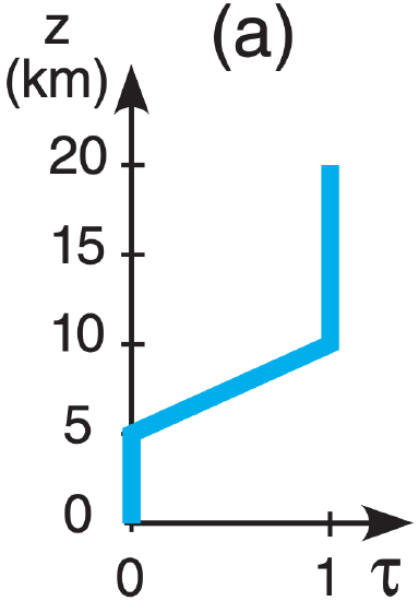
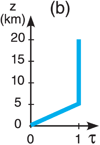
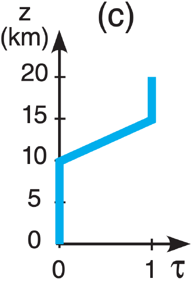
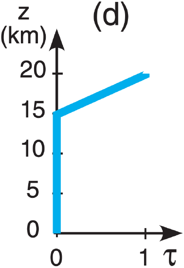
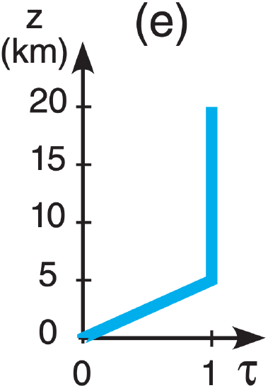
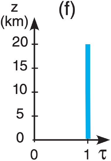
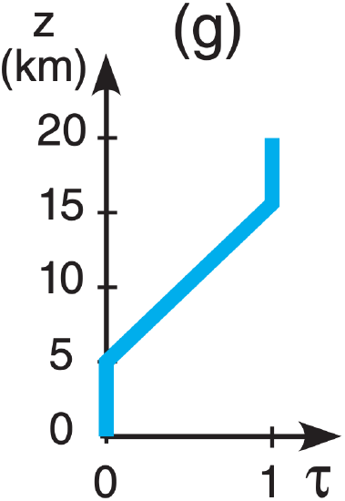
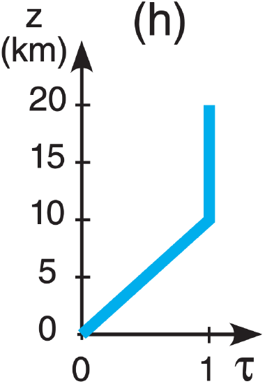
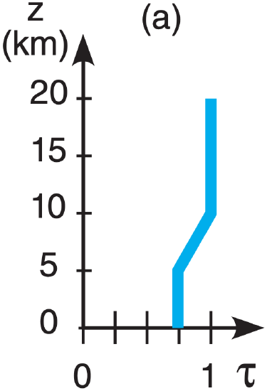
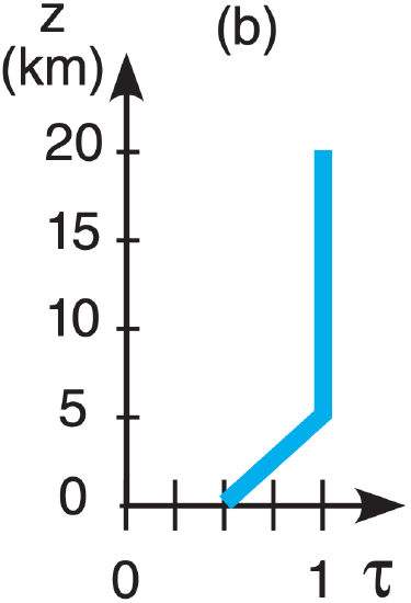
A5(§). Given the following temperature sounding:

z (km)	T (°C)	z (km)	T (°C)
15 to 20	–50	5 to 10	–5
10 to 15	–25	0 to 5	+5
		Earth skin	+20

Find the radiance at the top of the atmosphere for the following transmittance profiles & wavelengths:

λ (µm):	(a) 7.0 ,	(b) 12.7 ,	c) 14.4 ,	(d) 14.7
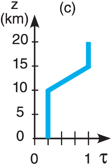
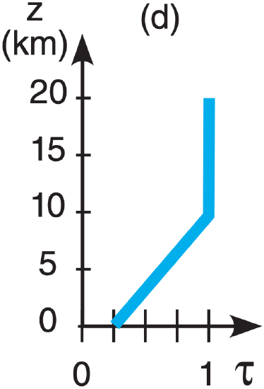
λ (µm):	(e) 11.0 ,	(f) 2.6 ,	(g) 6.5 ,	(h) 4.4

A6. For the transmittances of the previous exercise, plot the weighting functions.

A7. For the following altitudes (km) above the Earth’s surface, find the satellite orbital periods:

a. 40,000	b. 600	c. 800	d. 2,000	e. 5,000
f. 10,000	g. 15,000	h. 20,000	i. 30,000	j. 50,000

A8. What shade of grey would the following clouds appear in visible, IR, and water-vapor satellite images?

a. cirrus	b. cirrocumulus	c. cirrostratus	d. altocumulus	e. altostratus	f. stratus
g. nimbostratus	h. fog	i. cumulus humilis	j. cumulus congestus	k. cumulonimbus	l. stratocumulus

A9(§). Do an OSSE to calculate the radiances observed at the satellite, given the weighting functions of Fig. 8.20, but with the following atmospheric temperatures (°C): Layer 1 = –30, Layer 2 = –70, Layer 3 = –20, and Layer 4:

a. 40

b. 35

c. 30

d. 25

e. 20

f. 15

g. 10

h.5

A10. Find the beamwidth angle for a radar pulse for the following sets of [wavelength (cm) , antenna dish diameter (m)]:

a. [ 20, 8]	b. [20, 10]	c. [10, 10]	d. [10, 5]	e. [10, 3]
f. [5, 7]	g. [5, 5]	h. [5, 2]	i. [5, 3]	j. [3, 1]

A11. What is the name of the radar band associated with the wavelengths of the previous exercise?

A12. Find the range to a radar target, given the round-trip (return) travel times (µs) of:

a. 2	b. 5	c. 10	d. 25	e. 50
f. 75	g. 100	h. 150	i. 200	j. 300

A13. Find the radar max unambiguous range for pulse repetition frequencies (s^–1) of:

a. 50	b. 100	c. 200	d. 400	e. 600
f. 800	g. 1000	h. 1200	i. 1400	j. 1600

A14. Find the Doppler max unambiguous velocity for a radar with pulse repetition frequency (s^–1) as given in the previous exercise, for radar with wavelength of: (i) 10 cm (ii) 5 cm

A15. Determine the size of the radar sample volume at a range of 30 km for a 10 cm radar with 5 m diameter antenna dish and pulse duration (µs) of

a. 0.1

b. 0.2

c. 0.5

d. 1.0

e. 1.5

f. 2

g. 3

h. 5

A16(§). Calculate and plot the microwave refractivity vs. height using P and T of a standard atmosphere, but with vapor pressures (kPa) of:

a. 0	b. 0.05	c. 0.1	d. 0.2	e. 0.5
f. 1.0	g. 2	h. 5	i. 10	j. 20

[Note: Ignore supersaturation issues.]

A17(§). For the previous exercise, plot the vertical gradient ∆n/∆z of refractive index vs. height within the troposphere; determine the average vertical gradient in the troposphere; find the radius of curvature of the radar beam; and find the k_e beam curvature factor.

A18(§). For a radar with 0.5° elevation angle mounted on a 10 m tower, calculate and plot the height of the radar-beam centerline vs. range from 0 to 500 km, for the following beam curvature factors k_e, and name the type of propagation:

a. 0.5	b. 0.8	c. 1.0	d. 1.25	e. 1.33
f. 1.5	g. 1.75	h. 2	i. 2.5	j. 3

A19. Use the simple Z-R relationship to estimate the rainfall rate and the descriptive intensity category used by pilots and air traffic controllers, given the following observed radar echo dBZ values:

a. 10	b. 35	c. 20	d. 45
e. 58	f. 48	g. 52	h. 25

A20. Find reflectivity dBZ for rain 10 km from a WSR-88D, if received power (in 10^–14 W) is:

a. 1

b.2

c. 4

d. 6

e. 8

f. 10

g. 15

h. 20

i. 40

j. 60

k. 80

A21. Estimate the total rainfall accumulated in 1 hour, given the radar reflectivity values below:

Time (min)	dBZ	Time (min)	dBZ
0 - 10	15	29 - 30	50
10 - 25	30	30 - 55	18
25 - 29	43	55 - 60	10

A22. For an S-band radar (wavelength = 10 cm), what is the magnitude of the Doppler frequency shift, given radial velocities (m s^–1) of:

a. –110	b. –85	c. –60	d. –20
e. 90	f. 65	g. 40	h. 30

A23. Given a max unambiguous velocity of 25 m s^–1, what velocities would be displayed on a Doppler radar for rain-laden air moving with the following real radial velocities (m s^–1)?

a. 26	b. 28	c. 30	d. 35	e. 20	f. 25	g. 55
g. 55	h. –26	i. –28	j. –30	k. –35	l. –20

A24. Given a max unambiguous range of 200 km, at what range in the radar display does a target appear if its actual range is:

a. 205	b. 210	c. 250	d. 300	e. 350
f. 400	g. 230	h. 240	i. 390	j. 410

A25. Given the following sets of [average radial velocity (m s^–1) , range (km)], find the change of vertical velocity across a change of height of 1 km.

a. [–3, 100]	b. [–2, 200]	c. [–1, 50]	d. [–4, 50]
e. [3, 100]	f. [2, 200]	g. [1, 50]	h. [4, 50]

A26. Given polarimetric radar observations of Z_VV = 500 and Z_VH = 1.0, find the differential reflectivity and linear depolarization ratio for Z_HH values of:

a. 100	b. 200	c. 300	d. 400	e. 500
f. 600	g. 700	h. 800	i. 900	j. 1000

A27. Find the rainfall rate for the following sets of [K_DP (°/km) , Z_DR (dB)] as determined from polarimetric radar:

a. [1, 2]	b. [1, 3]	c. [1, 4]	d. [1, 5]
e. [2, 2]	f. [2, 6]	g. [3, 2]	h. [3, 4]
i. [3, 6]	j. [5, 2]	k. [5, 4]	l. [5, 6]

A28. A wind profiler has transmitters spaced 0.5 m apart. Find the beam zenith angle for ∆t (ns) of:

a. 0.2

b. 0.5

c. 1.0

d. 2

e. 3

f. 5

A29. For a wind profiler with 17° beam tilt, find U and W given these sets of [M_east(m s^–1), M_west(m s^–1)]:

a. [4, –4]	b. [4, –3]	c. [4, –5]	d. [–4, 4]
e. [–4, 3]	f. [–4, 5]	g. [1, 1]	h. [–1, –1]

8.5.3. Evaluate & Analyze

E1(§). Create blackbody radiance curves similar to Fig. 8.5, but for the following satellite channels. Does a monotonic relationship exists between brightness temperature and blackbody radiance?

1. GOES-16 channels 3 - 5.
2. Meteosat-10 imager channels 3 – 5
3. Meteosat-10 imager channels 6 - 8
4. GOES-15 sounder channels 1 - 4
5. GOES-15 sounder channels 5 - 8
6. GOES-15 sounder channels 9 - 12
7. GOES-15 sounder channels 13 - 16
8. GOES-15 sounder channels 17 - 18
9. Meteosat-10 imager channels 9 - 10

E2. For what situations would the brightness temperature NOT equal the actual temperature?

E3. a. Which GOES channels can see the Earth’s surface?

b. For the channels from part (a), how would the brightness temperature observed by satellite be affected, if at all, by a scene that contains scattered clouds of diameter smaller than can be resolved. For example, if the channel can see pixels of size 1 km square, what would happen if some of that 1 km square contained cumulus clouds of diameter 300 m, and the remaining pixel area was clear?

E4. Consider the radiative transfer equation. For an opaque atmosphere, \(\hat{\tau}_{\lambda \text { sfc }}=0\). What happens to the radiation emitted from the Earth’s surface?

E5. Knowing the relationship between transmittance profile and weighting function, such as sketched in Figs. 8.7 or 8.8, sketch the associated transmittance profile for the following GOES-15 sounder channels. [Hint, use the weights as sketched in Fig. 8.9 .]

a. 1	b. 2	c. 3	d. 4	e. 5
f. 6	g. 7	h. 10	i. 11	j. 12

E6(§). Given the following temperature sounding:

z (km)	T (°C)	z (km	T (°C)
15 to 20	–50	5 to 10	–5
10 to 15	–25	0 to 5	+5
		Earth skin	+20

Find the radiance at the top of the atmosphere for the following transmittance profiles & wavelengths:

λ (µm):	(a) 7.0 ,	(b) 12.7 ,	(c) 14.4 ,	(d) 4.4

[CAUTION: Transmittance ≠ 0 from the surface.]

E7. For the transmittances of the previous exercise, plot the weighting functions.

E8. a. How low an orbit can a LEO satellite have without the atmosphere causing significant drag?

[Hint, consider the exosphere discussion in the escape-velocity Info box in Chapter 1.]

b. What is the orbital period for this altitude?

c. If the satellite is too low, what would likely happen to it?

E9. a. What is the difference in orbital altitudes for geostationary satellites with orbital periods of 1 calendar day (24 h) and 1 sidereal day?

b. Define a sidereal day, explain why it is different from a calendar day, and discuss why the sidereal day is the one needed for geostationary orbital calculations.

E10. a. Discuss the meanings and differences between geostationary and sun-synchronous orbits.

b. Can satellite loops be made with images from polar orbiting satellites? If so, what would be the characteristics of such a loop?

c. What is the inclination of a satellite that orbits in the Earth’s equatorial plane, but in the opposite direction to the Earth’s rotation?

d. What are the advantages and disadvantages of sun-synchronous vs. geostationary satellites in observing the weather?

E11. What shade of grey would the following clouds appear in visible, IR, and water-vapor satellite images, and what pattern or shape would they have in the images?

1. jet contrail
2. two cloud layers: cirrus & altostratus
3. two cloud layers: cirrus & stratus
4. three cloud layers: cirrus, altostratus, stratus
5. two cloud layers: fog and altostratus
6. altocumulus standing lenticular
7. altocumulus castellanus
8. billow clouds
9. fumulus
10. volcanic ash clouds

E12. a. Using Fig. 8.8, state in words the altitude range that the plotted water-vapor channel sees.

b. Sometimes water-vapor satellite loops show regions becoming whiter with time, even though there is no advection of water vapor visible in the loop. What might cause this?

c. Why would very dense fog with 100% relative humidity invisible in that water-vapor satellite image?

E13(§). Re-do the temperature sounding retrieval exercise of Table 8-6 and its Sample Application. Iterate through each layer 3 times, and then discuss the answer and its errors. Start with an initial temperature (°C) guess at all heights of:

a. –60

b. –50

c. –40

d. –30

e. 0

f. Instead of an isothermal initial guess, use a different initial guess for each layer based on the standard atmosphere near the center of the layer.

E14. For locations (a) to (f) in the images below, interpret the following satellite images, taken by GOES12 at 2115 UTC on 18 Sept 2003, and justify your interpretation. Namely, indicate the cloud type (if any), its altitude, and or the weather feature.

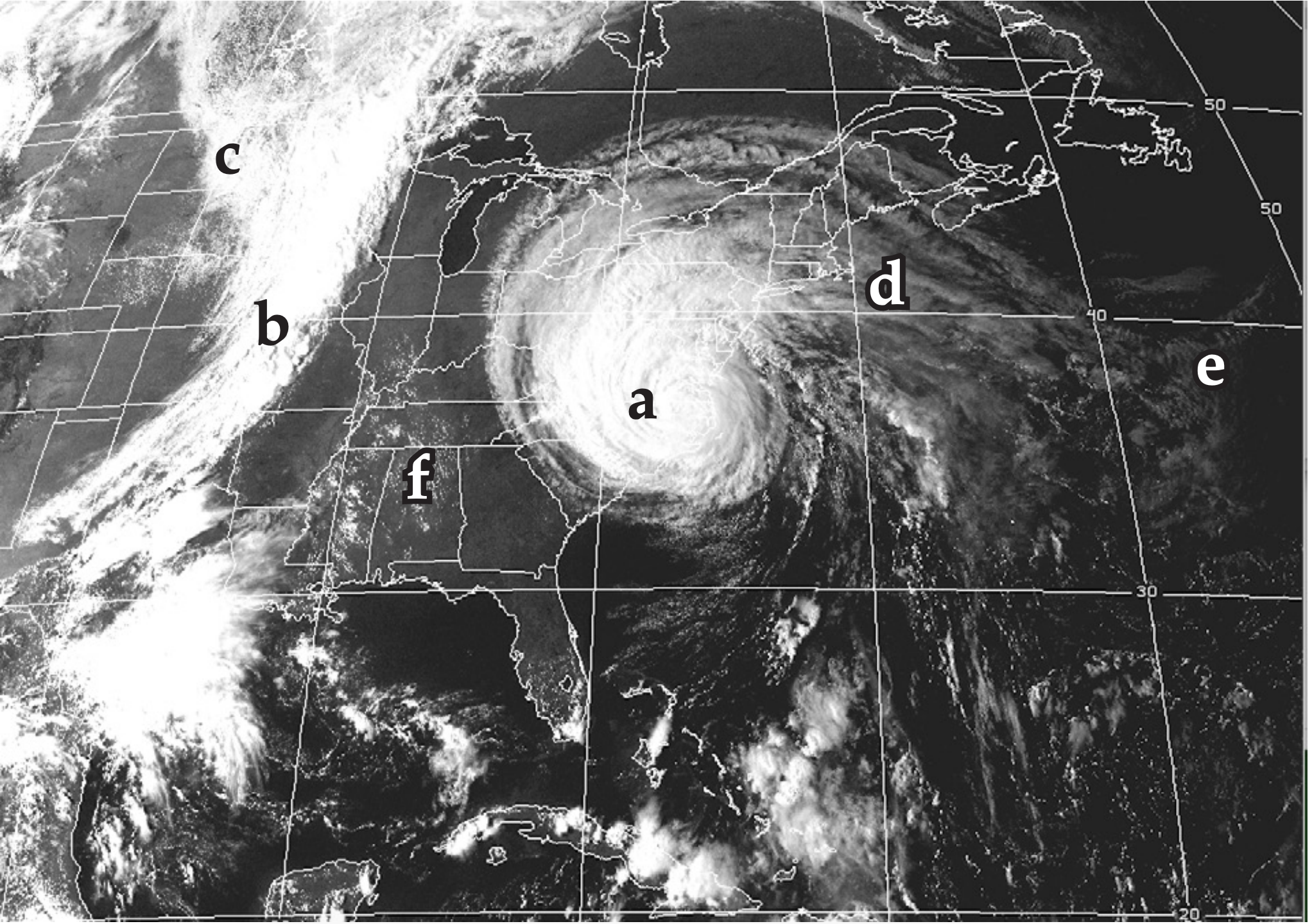
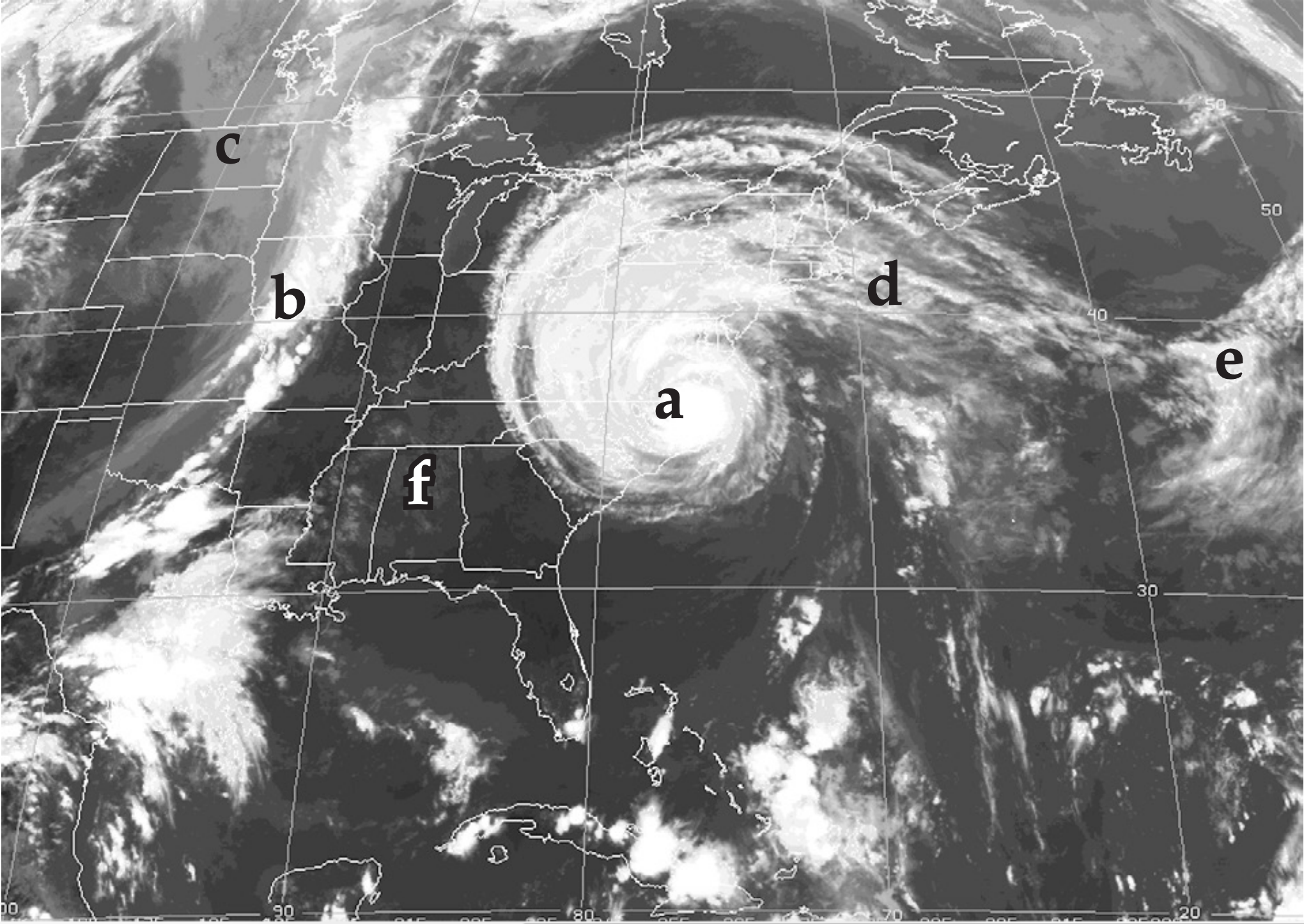
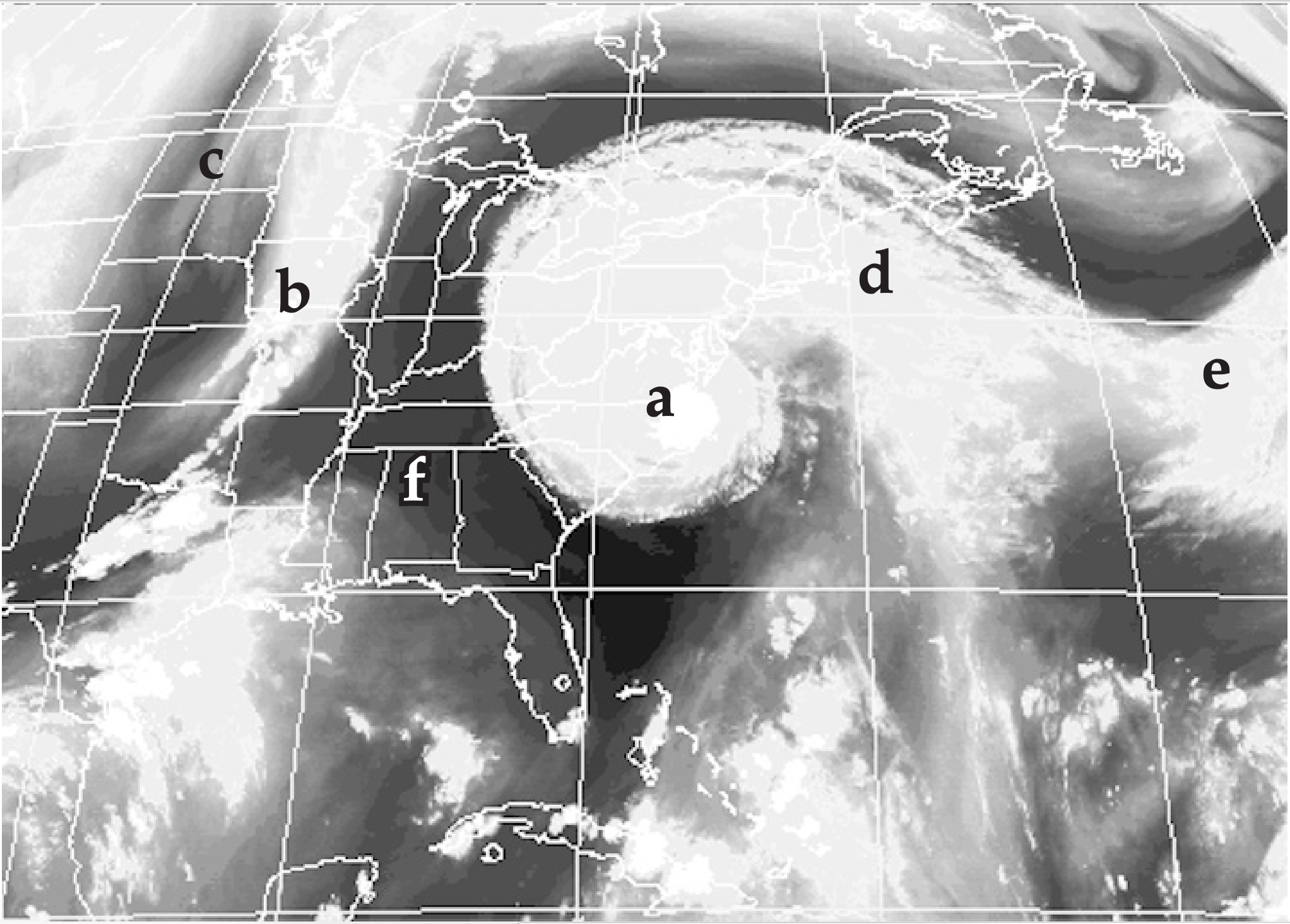
Top: visible. Middle: IR. Bottom: water vapor. (Images courtesy of Space Science & Engineering Center.)

E15(§). Re-do the temperature sounding retrieval exercise of Table 8-6 and its Sample Application. Iterate through each layer 3 times, and save your answer as a baseline result. Start with the same initial temperature (–45 °C) guess at all heights.

Then repeat the process with the following errors added to the radiances before you start iterating, and discuss the difference between these new results and the results from the previous paragraph. What is the relationship between radiance error measured by satellite and temperature sounding error resulting from the data inversion?

1. Channel 1, add 5% error to the radiance.
2. Channel 1, subtract 5% error from radiance.
3. Channel 2, add 5% error to the radiance.
4. Channel 2, subtract 5% error from radiance.
5. Channel 3, add 5% error to the radiance.
6. Channel 3, subtract 5% error from radiance.
7. Channel 4, add 5% error to the radiance.
8. Channel 4, subtract 5% error from radiance.

E16(§). For Doppler radar, plot a curve of R_max vs. M_{r max} for a variety of PRFs between 100 and 2000 s^–1 , identify the problems with the interpretation of velocities and ranges above and below your curve, and discuss the Doppler dilemma. Use the following Doppler radar wavelengths (cm) for your calculations, and identify the name of their radar band:

a. 20

b. 10

c. 5

d. 3

e. 2

f. 1

E17. Discuss the advantages and disadvantages of PPI, CAPPI, RHI, and AVCS displays for observing:

a. thunderstorms

b. hurricanes

c. gust fronts

d. low-pressure centers

e. fronts

E18(§). For P = 90 kPa, calculate a table of values of ∆N/∆z for different values of temperature gradient ∆T/∆z along the column headers, and different values of ∆e/∆z along the row headers. Then indicate beam propagation conditions (superrefraction, etc.) in each part of the table. Suggest when and where the worst anomalous propagation would occur.

E19. Which is more important in creating strong radar echoes: a larger number of small drops, or a small number of larger drops? Why?

E20. Derive eq. (8.31) using the geometry of a spherical drop.

E21. For radar returns, explain why is the log(range) includes a factor of 2 in eq. (8.28).

E22. By what amount does the radar reflectivity factor Z change when dBZ increases by a factor of 2?

E23. Hong Kong researchers have found that Z = a₃·RR^a4, where a₃ = 220 ±12 and a₄ = 1.33 ±0.03, for RR in mm h^–1 and Z in mm⁶ m^–3. Find the corresponding equation for RR as a function of dBZ.

E24. Why (and under what conditions) might a weather radar NOT detect cells of heavy rain, assuming that the radar is in good working condition?

E25. How might the bright band look in the vertical velocities measured with a wind profiler? Why?

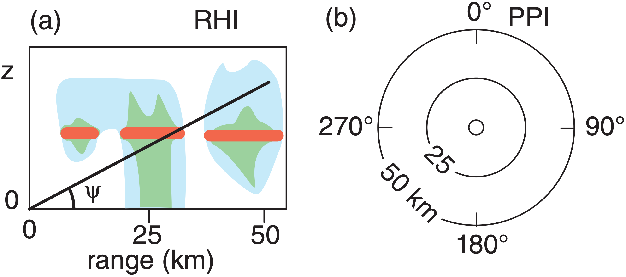
E26. Given an RHI radar display showing a bright band (see Fig. a below). If the radar switches to a PPI scan having elevation angle ψ shown in (a), sketch the appearance of this bright band in Fig. b. Assume the max range shown in (a) corresponds to the largest range circle drawn in (b).

Fig. RHI radar display (a), showing echoes from precipitation regions (shaded). Bright-band echoes are the darker grey horizontal lines. Draw your answer in the blank PPI display of Fig. b.

E27. What design changes would you suggest to completely avoid the limitation of the max unambiguous velocity?

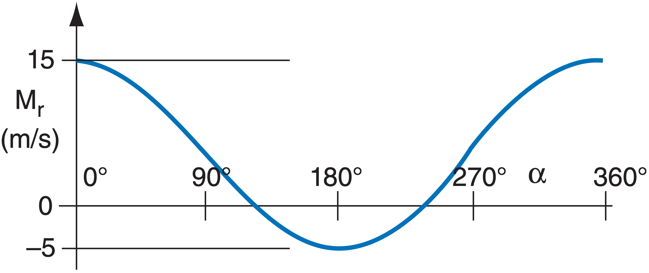
E28. Interpret the VAD display below to diagnose mean wind speed, direction, & convergence, if any.

E29(§). Create a table of rainfall rate values, where each column is a different K_DP value (within typical range), and each row is a different Z_DR value. Draw the isohyets by hand in that table (i.e., draw lines connecting points of equal rainfall rate).

E30. Discuss the advantages and disadvantages of using larger zenith angle for the beams in a wind profiler.

E31. a. Given the vectors drawn in Fig. 8.44, first derive a equations for M_east and M_west as the sum of the wind vectors projected into the east and west beams, respectively. Then solve those coupled equations to derive eqs. (8.42).

b. Write eqs. similar to eq. (8.42), but for the V and W winds based on M_north and M_south.

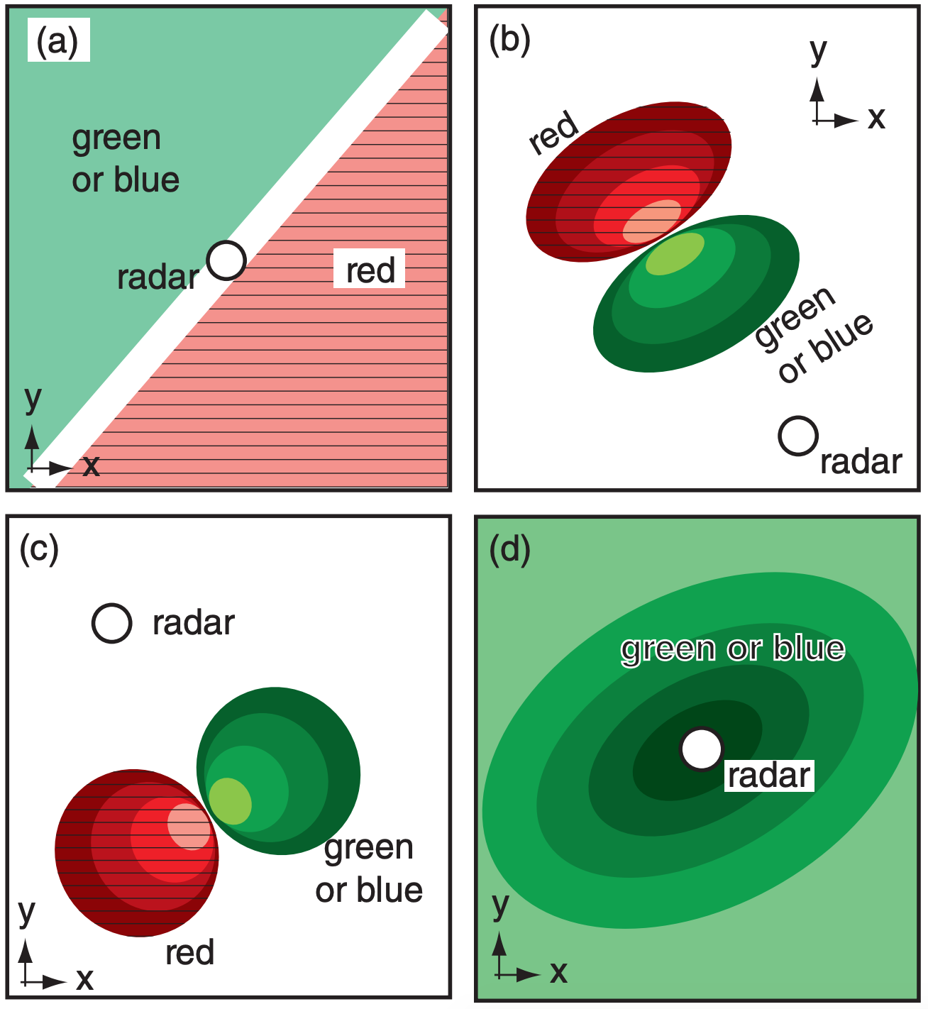
E32. Interpret the weather conditions sketched in the figures below as could be observed on a Doppler radar display of radial velocity.

8.5.4. Synthesize

S1. What if substantial cloud coverage could occur at any depth in the stratosphere as well as in the troposphere. Discuss how clouds at different altitudes would look in visible, IR, and water-vapor satellite images. Are there any new difficulties?

S2. What if molecular scattering by air was significant at all wavelengths. How would that affect satellite images and sounding retrievals, if at all?

S3. Suppose that Planck’s law and brightness temperature were not a function of wavelength. How would IR satellite image interpretation be affected?

S4. If satellite weighting functions have about the same vertical spreads as plotted in Fig. 8.9, discuss the value of adding more and more channels.

S5. What if gravity on Earth were twice as strong as now. What would be the altitude and orbital period of geostationary satellites?

S6. What if the Earth were larger diameter, but had the same average density as the present Earth. How large would the diameter have to be so that an orbiting geostationary weather satellite would have an orbit that is zero km above the surface? (Neglect atmospheric drag on the satellite.)

S7. Determine orbital characteristics for geostationary satellites over every planet in the solar system.

S8. What if you could put active radar and lidar on weather satellites. Discuss the advantages and difficulties. (Note, this is actually being done.)

S9. Devise a method to eliminate both the max-unambiguous range and max-unambiguous velocity of Doppler radar.

S10. What if pressure and density were uniform with height in the atmosphere. How would radar beam propagation be affected?

S11. Compile (using web searches) the costs of developing, launching, operating, and analyzing the data from a single weather satellite. Compare with analogous costs for a single rawinsonde site.

S12. What if radar reflectivity was proportional only to the number of hydrometeors in a cloud, and not their size. How would radar-echo displays and rainfall-rate calculations be affected?

S13. What if Doppler radars could measure only tangential velocity rather than radial velocity. Discuss how mean wind, tornadoes, and downburst/ gust-fronts would look to this radar.

S14. Radio Acoustic Sounding Systems (RASS) are wind profilers that also emit loud pulses of sound waves that propagate vertically. How can that be used to also measure the temperature sounding?