
8.8: Can the Eulerian and Lagrangian frameworks be connected?
- Page ID
- 5608
\[R=R(x,y,z,t)\]
To find the change in the rainfall rate R in an air parcel over space and time, we can take its differential, which is an infinitesimally small change in R:
\[d R=\frac{\partial R}{\partial t} d t+\frac{\partial R}{\partial x} d x+\frac{\partial R}{\partial y} d y+\frac{\partial R}{\partial z} d z\]
where dt is an infinitesimally small change in time and dx, dy, and dz are infinitesimally small changes in x, y, and z coordinates, respectively, of the parcel.
If we divide Equation [8.15] by dt, this equation becomes:
\[\frac{d R}{d t}=\frac{\partial R}{\partial t}+\frac{\partial R}{\partial x} \frac{d x}{d t}+\frac{\partial R}{\partial y} \frac{d y}{d t}+\frac{\partial R}{\partial z} \frac{d z}{d t}\]
where dx/dt, dy/dt, and dz/dt describe the velocity of the air parcel in the x, y, and z directions, respectively.
Let’s consider two possibilities:
Case 1: The air parcel is not moving. Then the change in x, y and z are all zero and:
\[\frac{d R}{d t}=\frac{\partial R}{\partial t}\]
So, the change in the rainfall rate depends only on time. \(\frac{\partial R}{\partial t}\) is called the Eulerian or local time derivative. It is the time derivative that each of our weather observing stations record.
Case 2: The air parcel is moving. Then the changes in its position occur over time, and it moves with a velocity, \(\vec{U}=\vec{i} u+\vec{j} v+\vec{k} w,\) where:
\[\frac{d x}{d t}=u \quad \frac{d y}{d t}=v \quad \frac{d z}{d t}=w\]
\[\frac{d R}{d t}=\frac{\partial R}{\partial t}+u \frac{\partial R}{\partial x}+v \frac{\partial R}{\partial y}+w \frac{\partial R}{\partial z}\]
A special symbol is given for the derivative when you follow the air parcel around. It is called the substantial, or total, derivative and is denoted by:
\[\frac{D R}{D t}=\frac{\partial R}{\partial t}+u \frac{\partial R}{\partial x}+v \frac{\partial R}{\partial y}+w \frac{\partial R}{\partial z}\]
Mathematically, we can express this equation in a more general way by thinking about the dot product of a vector with the gradient of a scalar as we did in an example of the del operator:
\[\frac{D R}{D t}=\frac{\partial R}{\partial t}+\vec{U} \cdot \vec{\nabla} R\]
where the second term on the right hand side is called the advective derivative, which describes changes in rainfall that are solely due to the motion of the air parcel through a spatially variable rainfall distribution.You should be able to show that equation [8.19] is the same as equation [8.18].
We can rearrange this equation to put the local derivative on the left.
\[\frac{\partial R}{\partial t}=\frac{D R}{D t}-\vec{U} \cdot \vec{\nabla} R\]
The term on the left is the local time derivative, which is the change in the variable R at a fixed observing station. The first term on the right is the total derivative, which is the change that is occurring in the air parcel as it moves. The last term on the right, \(-\vec{U} \cdot \vec{\nabla} R,\) is called the advection of \(R\) , Note that advection is simply the negative of the advective derivative.
To go back to the analogy of the thunderstorm, the change in rainfall that you observed driving in your car was the total time derivative and it depended only on the change in the intensity of the rain in the thunderstorm. However, for each observer in a house, the change in rainfall rate depended not only on the intensity of the rainfall as the thunderstorm was over the house but also on the movement of the thunderstorm across the landscape.
R can be any scalar. Rainfall rate is one example, but the most commonly used are pressure and temperature.
Equation [8.20] is called Euler’s relation and it relates the Eulerian framework to the Lagrangian framework. The two are related by this new concept called advection.
Let’s look at advection in more detail, focusing on temperature.
We generally think of advection being in the horizontal. So often we only consider the changes in the x and y directions and ignore the changes in the zdirection:
horizontal temperature advection \[=-\vec{U}_{H} \cdot \vec{\nabla}_{H} T=-\left(u \frac{\partial T}{\partial x}+v \frac{\partial T}{\partial y}\right)\]
So what’s with the minus sign? Let’s see what makes physical sense. Suppose Tincreases only in the x-direction so that:
\[\frac{\partial T}{\partial y}=0\) and \(\frac{\partial T}{\partial x}>0\]
If u > 0 (westerlies, blowing eastward), then both u and \(\frac{\partial T}{\partial x}\) are positive so that temperature advection is negative. What does this mean? It means that colder air blowing from the west is replacing the warmer air, and the temperature at our location is getting decreasing from this advected air. Thus \(\frac{\partial T}{\partial t}\) should be
negative since time is increasing and temperature is decreasing due to advection.
If the temperature advection is negative, then it is called cold-air advection, or simply cold advection. If the temperature advection is positive, then it is called warm-air advection, or simply warm advection.
Some examples of simple cases of advection show these concepts (see figure below). When the wind blows along the isotherms, the temperature advection is zero (Case A). When the wind blows from the direction of a lower temperature to a higher temperature (Case B), we have cold-air advection. When the wind blows as some non-normal direction to the isotherms, then we need to multiply the magnitude of the wind and the temperature gradient by the cosine of the angle between them. We can estimate the temperature advection by doing what we did for the gradient, that is, replace all derivatives and partial derivatives with finite Δs.
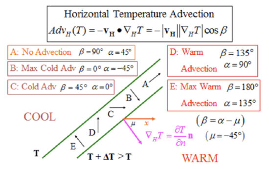
Credit: H.N. Shirer
When the isotherms with the same temperature difference are further apart on the map (see figure below), then the horizontal temperature advection will be less than when the isotherms are closer together, if the wind velocity is the same in the two cases.
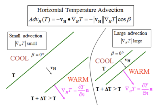
Credit: H.N. Shirer
In summary, to calculate the temperature advection, first determine the magnitude and the direction of the temperature gradient. Second, determine the magnitude and direction of the wind. The advection is simply the negative of the dot product of the velocity and the temperature gradient.
Watch this video (2:20) on calculating advection:
Finding Advection
- Click here for transcript of the Finding Advection video.
-
Temperature advection is just a dot product of the velocity vector and the temperature gradient vector at that point. Let's choose this point in Pennsylvania where we've already calculated the gradient of this point. Let's look at the wind vector. So the station weather plot has a wind barb that's northwesterly and five knots. And so we can estimate, since this is x direction, and since this is north, we can estimate that this is about 300 degrees in terms of meteorology angle. So to find the math angle, which is what we need for the calculation here, we need to take 270 degrees. And we subtract 300 degrees from that, and we get alpha equals minus 30, which is 330 degrees if we start from the x-axis and we go counterclockwise all the way around to this direction like this. We've already figured out that the gradient has an angle that's 301 degrees, and that's from the x-axis going all the way around. So that's something like this. And therefore, the difference between the two is 29 degrees. And that's beta. We know that the magnitude of the temperature gradient is 0.12 degrees Fahrenheit. So we multiply the magnitude of the velocity times the magnitude of the temperature gradient times cosine of 29 degrees. We end up getting a value of 0.52 and the minus sign degrees Fahrenheit per hour. So the minus sign is here, because this is positive, positive, and positive. And so the advection is minus 0.52 degrees Fahrenheit per hour. This is cold air advection, or cold advection.
Quiz 8-4: The advection connection.
- Find Practice Quiz 8-4 in Canvas. You may complete this practice quiz as many times as you want. It is not graded, but it allows you to check your level of preparedness before taking the graded quiz.
- When you feel you are ready, take Quiz 8-4. You will be allowed to take this quiz only once. Good luck!