
11.8: Here’s How Reynolds Did Averaging
- Page ID
- 3422

For any variable, the observed value can be written as a sum of the mean value and a turbulent value:
\[u=\bar{u}+u^{\prime}\]
where \(\bar{u}\) is the mean, or average value, and \(u^{\prime}\) is the turbulent part.
The average can be obtained by averaging \(u\) over time or over space or even by doing a number of samples and averaging over the samples.
- temporal averaging: \[\bar{u}=\dfrac{\int u(t) d t}{\int d t}=\dfrac{\sum_{i=0}^{N-1} u\left(t_{i}\right)}{N}\]
- spatial averaging: \[\bar{u}=\dfrac{\int u(x) d x}{\int d x}=\dfrac{\sum_{i=0}^{N-1} u\left(x_{i}\right)}{N}\]
If the turbulence does not change with time and is homogeneous (i.e., the same in all directions and for all time), then these averages equal each other.
In Lesson 10, we developed the equation of motion without really considering the short-term and small-scale variations, except to say that they led to turbulent drag, which acts to resist the mean flow in the upper boundary layer. Now we want to think about how to correctly capture the dynamic effects of turbulent motion. What we want to do is to write down the equations of motion that you learned in Lesson 10; substitute mean and turbulent parts for the variables such as u, v, and w; average over all the terms; and then see if we can sort out the terms to create an equation for the mean wind and an equation for the turbulent wind. This type of averaging is called Reynolds averaging.
But first we need to learn the rules for averaging.
Rules of Averaging
c is constant; u and v are variables
\[\overline{u^{\prime}}=0\]
\[\overline{c u}=c \bar{u}\]
\[\overline{u+v}=\bar{u}+\bar{v}\]
\[\overline{(\bar{u} v)}=\bar{u} \bar{v}\]
\[\overline{\left(\frac{\partial u}{\partial t}\right)}=\frac{\partial \bar{u}}{\partial t}\]
Now let’s apply these rules to a variable with a mean and a turbulent part. For example, consider the product uv, which is just the advection of horizontal wind in one direction by the horizontal wind in the other direction.
So, using the rules:
\[\begin{aligned} \overline{u v} &=\overline{\left(\bar{u}+u^{\prime}\right)\left(\bar{v}+v^{\prime}\right)} \\ &=\overline{\bar{u}} \bar{v}+\overline{\bar{u} v^{\prime}}+\overline{u^{\prime} \bar{v}}+\overline{u^{\prime} v^{\prime}} \end{aligned}\]
and
\[\overline{\overline{u v}}=\bar{u} \bar{v}\]
\[\overline{\bar{u} v^{\prime}}=\bar{u} \overline{v^{\prime}}=\bar{u} \cdot 0=0\]
\[\overline{u^{\prime} \bar{\nu}}=\overline{u^{\prime} \bar{\nu}}=0 \cdot \bar{\nu}=0\]
so
\[\overline{u v}=\bar{u} \bar{v}+\overline{u^{\prime} v^{\prime}}\]
This second term, a product of two turbulent terms is not necessarily zero! Whereas the average of one turbulent term is zero by definition, the average of two turbulent terms is not necessarily zero.
The following video (3.11) further describes Reynolds averaging:
Reynold's Averaging
- Click here for transcript of the Reynold's Averaging.
-
Reynold's averaging is really pretty straightforward once you understand the rules. Each variable has an average and a perturbation, or turbulent, part. We need to determine the time over which we want to find the average. But after we do that, we can average all the values and then subtract the average from each individual value in order to find the perturbed or turbulent or fluctuation part of that value. The average the average value is, of course, the same for all the values in the average. I will use the words "mean" and "average" interchangeably for the noun meaning average. And we'll use the words like perturbation, fluctuation, and turbulent part to describe the variations of individual values about the average value. The rules are pretty simple. First, the average of a perturbed or turbulent term is 0, because if it were not, then the average value would be incorrect. Second, the average of the product of a constant times a variable is just a product of the average of the constant times the average of the variable. The average of the sum of two variables is just the sum of the average of the two variables. And the average of a product of the average value of one variable and another variable is just a product of the averages of the two variables. Note that the average of a variable is just a constant. Be careful. We will soon see that the average of the product of two variables is not just the product of the average of two variables. Finally, the average of the derivative of a variable is just a derivative of the average of the variable. Let's calculate the Reynold's average of one term of the equation for kinetic energy, which is just 1/2 mv squared. If we divide by the air density, then we have the kinematic kinetic energy. Each term can be written as its mean in turbulent parts. Let's look only at the u term. The v and w terms can be calculated in the same way. So we multiply all the terms out, then take the Reynold's average and apply the rules. Average values of average values are just average values. Because an average value is a constant, we get two terms of a constant times the average of the perturbed term, which is just 0. When we are done, we see that we have two terms left-- the average u squared, and the perturbation term squared. You can make a simple model with a random number generator to demonstrate the average of the product of two perturbation terms is not necessarily 0. This calculation was chosen so that the averages for u and v were 0. And so the average of the product of average u and average v is 0, but the average of the perturbations is not 0.
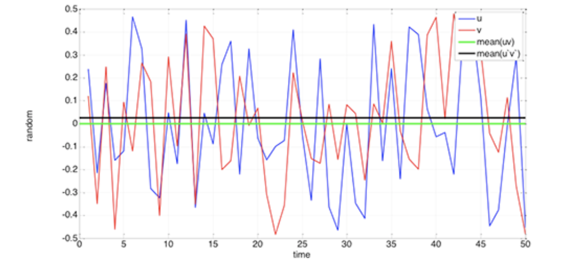
Example \(\PageIndex{1}\)
Consider two random numbers varying between –0.5 and 0.5, called u and v. The figure below shows u, v, the mean of uv and the mean of u’v’. Of course, the mean of u’v’ might be zero, but is it not necessarily zero, as shown in this figure.
The same thinking applies to u2.
\[\overline{u^{2}}=\overline{\left(\bar{u}+u^{\prime}\right)\left(\bar{u}+u^{\prime}\right)}=\ldots=\bar{u}^{2}+\overline{u^{\prime 2}}\]
Remember your statistics and the concept of variance:
\[\sigma_{u}^{2}=\frac{1}{N-1} \sum_{i=0}^{N-1}\left(u_{i}-\bar{u}\right)^{2} \approx \frac{1}{N} \sum_{i=0}^{N-1}\left(u_{i}-\bar{u}\right)^{2}=\frac{1}{N} \sum_{i=0}^{N-1}\left(u_{i}^{\prime}\right)^{2}=\overline{u^{2}}\]
So, the variance is the same as the mean value for the square of the turbulent part of the variable.
The covariance of u and v is given by the equation:
covariance \[(u, v)=\overline{u^{\prime} v^{\prime}}\]
We can get a better sense of how large this variance is by dividing by the mean value:
\[\mathrm{I}=\frac{\sigma_{u}}{\bar{u}}\]