6.1: Front Matter

What Is An Earthquake?

An earthquake is a sudden shaking of the ground primarily as a result of fault movement. However, volcanic activity, landslides, impacts, or even human-induced activity can trigger an earthquake. Earthquakes have been experienced by humans throughout our short history. Most ancient cultures developed myths to explain them, including envisioning large creatures - gods or goddesses - within Earth moving to create the quake.

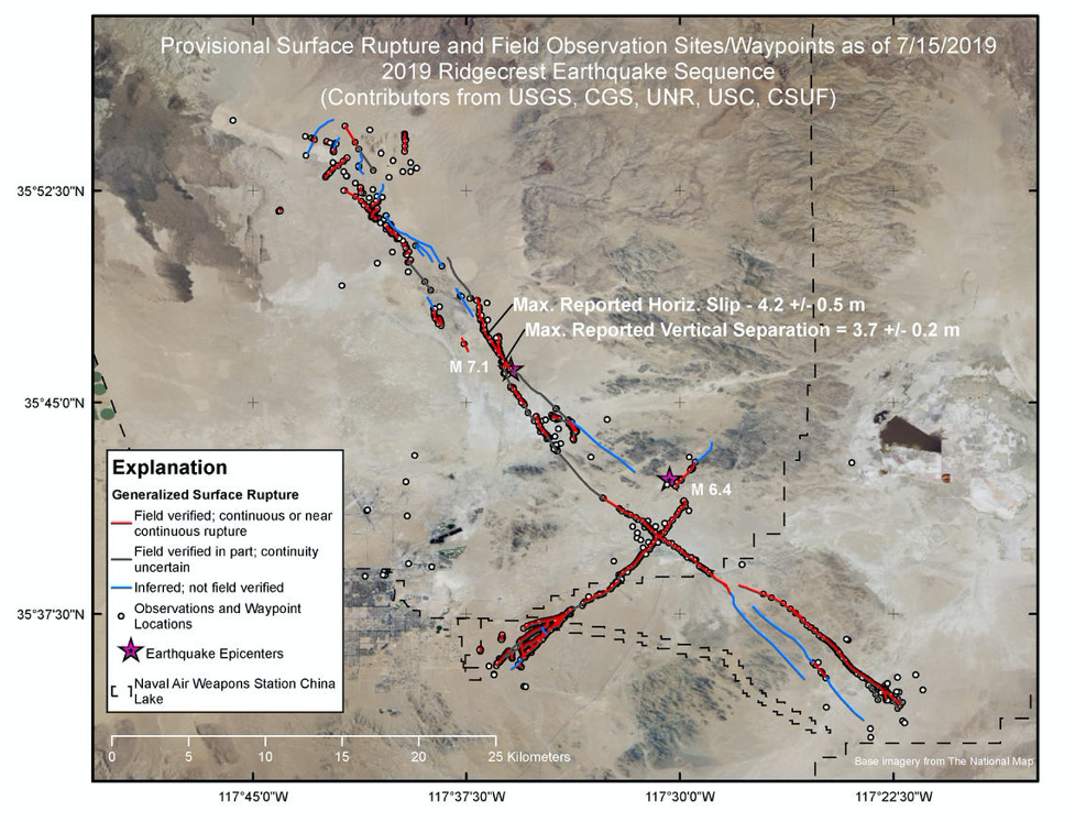
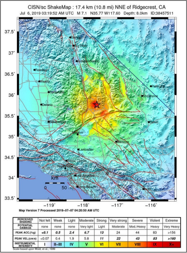
On July 5, 2019, a 7.1 magnitude earthquake hit Ridgecrest, California. This was the main shock of the sequence; the previous day, a 6.4 magnitude foreshock (smaller earthquakes that precede the main earthquake) occurred. Both earthquakes were felt over a wide area of Southern California. Thousands of aftershocks (smaller earthquakes that follow a larger earthquake) have occurred since (Figure 6.1).

Figure 6.1: General surface rupture based on field mapping and satellite data as of July 15, 2019. Ruptures from the magnitude 6.4 event trend northeast to southwest, and ruptures from the magnitude 7.1 event trend northwest to southeast. Circles indicate where scientists have visited the fault surface.

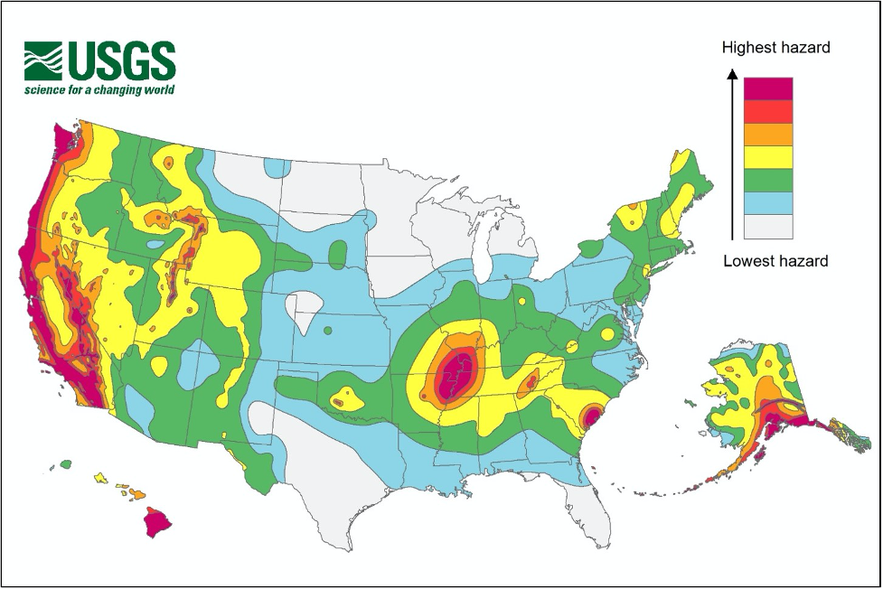
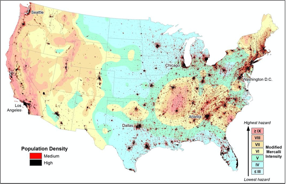
California is no stranger to earthquakes. We have many faults and fault systems throughout the state, including the infamous San Andreas Fault. Many of our faults are a consequence of California’s position on a tectonic plate boundary. Most earthquakes (95%) occur along plate boundaries, while the remaining 5% occur in the interior of a tectonic plate (intraplate). In North America, most earthquakes occur along the West Coast in association with plate boundaries, but intraplate earthquakes occasionally occur in places like the New Madrid, Missouri area (Figure 6.2).

Figure 6.2: Earthquake hazard map showing peak ground accelerations having a 2 percent probability of being exceeded in 50 years, for a firm rock site. The map is based on the most recent USGS models for the conterminous U.S. (2018), Hawaii (1998), and Alaska (2007). The models are based on seismicity and fault-slip rates and consider the frequency of earthquakes of various magnitudes. Locally, the hazard may be greater than shown, because site geology map amplify ground motions.

Earthquakes provide valuable information about conditions in Earth’s interior and at the surface. And, unlike previous topics we’ve explored, earthquakes are a hazard with inherent risks to human society. Those of us in California likely have experienced at least one earthquake in our lifetime (maybe more!). Therefore, we are aware of the need to consider hazard mitigation, including planning, preparation, and communication, all commonly supported by the science of seismology.

Figure 6.3

Seismologists and geophysicists are the primary investigators of earthquakes; however, other geoscientists may study them, as well. Like many other geoscientists, working with other disciplines is common, with a heavy influence from both math and technology. Many are employed by universities where they teach and/or do research, and state and federal agencies, including geological surveys, like the California Geological Survey or United State Geological Survey (USGS). Additional career pathways are available in the private sector including in mining and natural resource extraction or in hazard mitigation and assessment. Many of these career options require a college degree and postgraduate work. If you are interested, talk to your geology instructor for advice. We recommend completing as many math and science courses as possible (chemistry is incredibly important for mineralogy). Also, visit National Parks, CA State Parks, museums, gem & mineral shows, or join a local rock and mineral club. Typically, natural history museums will have wonderful displays of rocks, including those from your local region. Here in California, there are a number of large collections, including the San Diego Natural History Museum, Natural History Museum of Los Angeles County, Santa Barbara Museum of Natural History, and Kimball Natural History Museum. Many colleges and universities also have their own collections/museums.

Earthquake Focus, Epicenter, and Waves

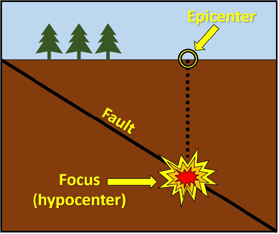
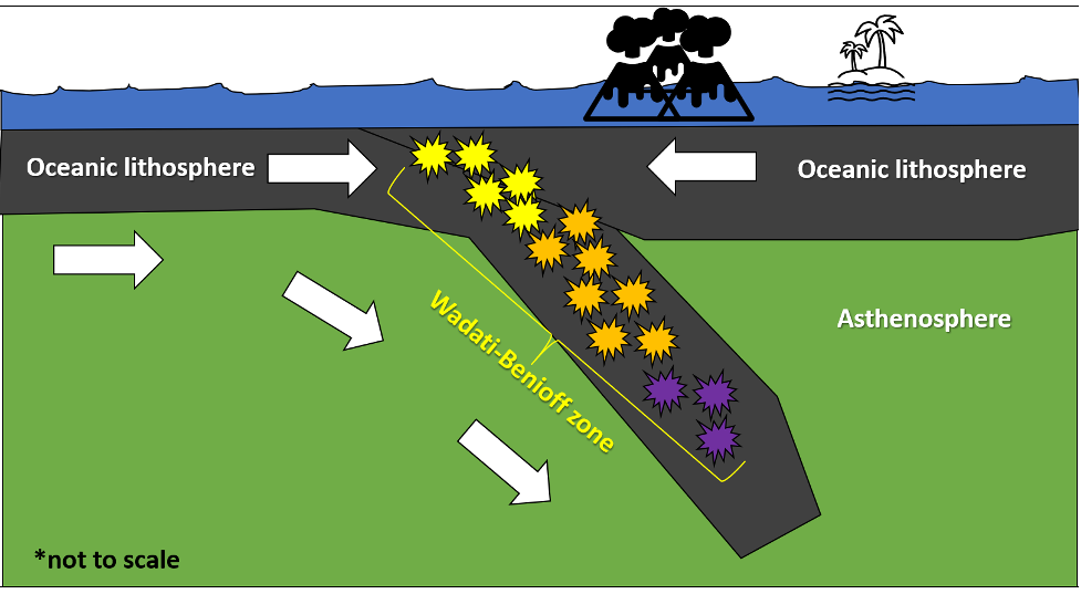
Earthquakes originate at a point called the focus (plural foci) or hypocenter. From this point, energy travels outward in different types of waves. The place on the Earth’s surface directly above the focus is called the epicenter (Figure 6.4). Earthquake foci may be shallow (less than 45 miles from Earth’s surface) to deep (greater than 185 miles deep), though shallow to intermediate depths are much more common. Earthquake frequency and depth are related to plate boundaries. The vast majority (95%) of earthquakes occur along a plate boundary, with shallow focus earthquakes tending to occur at divergent and transform plate boundaries, and shallow, intermediate, and deep focus earthquakes occurring at convergent boundaries (along the subducting plate). The earthquakes associated with convergent boundaries occur along Wadati-Benioff zones, or simply Benioff zones, areas of dipping seismicity along the subducting plate (Figure 6.5).

Figure 6.4: An illustration depicting the focus, where the earthquake originates, and the epicenter, the point on the ground’s surface directly above the focus.

 

Figure 6.5: An illustration depicting a subduction zone with associated Wadati-Benioff Zone.

Earthquake Waves

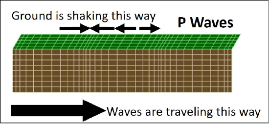
As an earthquake occurs, two different types of waves are produced: 1) body waves, so termed because they travel through the body of the Earth, and 2) surface waves that travel along the Earth’s surface. There are two types of body waves: P-waves and S-waves. P-waves, or primary waves, are compressional waves that move back and forth, like the action of an accordion. As the wave passes, the atoms in the material it is travelling through are compressed and stretched (Figure 6.6). Movement is compressional parallel to the direction of wave propagation, which makes P-waves the fastest of the seismic waves. These waves can travel through solids, liquids, and gases, because all materials can be compressed to some degree.

Figure 6.6: P-wave and their general movement through a rock body.

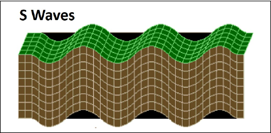
S-waves, or secondary waves, are shear waves that move material in a direction perpendicular to the direction of travel (Figure 6.7). S-waves can only travel through solids and are slightly slower than P-waves. Think of a wave movement like the wave created by fans in a stadium that stand up and sit down. Body waves are often responsible for the jerking and shaking motions felt during an earthquake.

Figure 6.7: S-wave and their movement through a rock body.

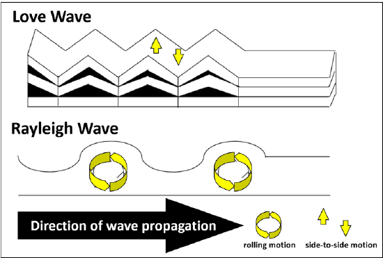
Surface waves, which are only propagated along the surface of the Earth, are slower than body waves. Additionally, their movement is often not handled by buildings well, so these waves are responsible for considerable damage to structures. These waves move slowly, which often results in an increase in amplitude. Love waves are the faster surface waves, and they move material back and forth in a horizontal plane that is perpendicular to the direction of wave travel (Figure 6.8). Rayleigh waves make the Earth’s surface move in an elliptical, rolling motion, like the movement in an ocean wave (Figure 6.8). Combined, this results in ground movement that is both up and down and side-to-side.

Figure 6.8: Love and Rayleigh wave propagation.

Table 6.1: Summary table of the different seismic waves and their arrival order to a distance seismic station

Category	Type	Average velocity through the crust (miles per second)	Arrival placement at distant seismogram
Body	Primary (P)	5 mi/s	First
Body	Secondary (S)	3 mi/s	Second
Surface	Love (L)	2.8 mi/s	Third
Surface	Rayleigh (R)	2.2 mi/s	Fourth

Want to view seismic waves in action? Visit the Incorporated Research Institutions for Seismology (IRIS) for videos showing wave motion.

Recording Earthquakes

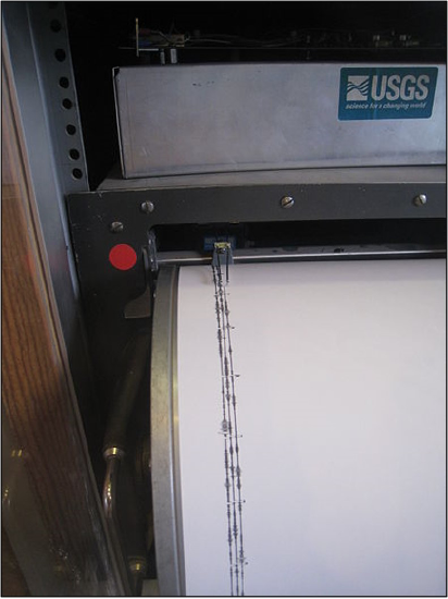
The formal study of earthquakes, called seismology, began with the development of instruments that were capable of detecting earthquakes. This instrument, called a seismograph or seismometer, can measure the slightest of Earth’s vibrations (Figure 6.9). A typical seismograph consists of a mass suspended on a string from a frame that moves as the Earth’s surface moves. A rotating drum is attached to the frame, and a pen attached to the mass, so that the relative motion is recorded in a seismogram (Figure 6.10). It is the seismograph frame, attached to the ground, that moves during an earthquake. The suspended mass generally stays still due to inertia.

Figure 6.9: A USGS seismograph at the Point Reyes visitor center, near the San Andreas Fault.

 

Figure 6.10: The P-waves are the first to arrive at each station, followed by the S-waves. Because the P-waves travel faster than S-waves the great distance between the two (S-P interval), the further away the earthquake epicenter.

 

How Are Earthquakes Measured?

The tragic consequences of earthquakes can be measured in many ways, like death tolls or force of ground shaking. However, there are two measures that are commonly used. One is a qualitative measure of the damage inflicted by the earthquake, referred to as intensity. The second is a quantitative measure of the energy released by the earthquake, termed magnitude. Both measures provide meaningful data.

Earthquake Intensity

Intensity measurements consider both the damage incurred due to the quake and the way that people respond to it. The Modified Mercalli Intensity Scale (Table 6.2) is the most widely used scale to measure earthquake intensities. This scale has values that range from Roman numerals I to XII that characterize the damage observed and people’s reactions to the shaking.

Table 6.2: The Modified Mercalli Intensity scale, roman numeral rankings and their associated characteristics.

Modified Mercalli Intensity Scale
Intensity	Characteristics
I	Shaking is not felt under normal circumstances.
II	Shaking felt only by those at rest, mostly along upper floors in buildings.
III	Weak shaking felt noticeably by people indoors. Many do not recognize this as an earthquake. Vibrations like a large vehicle passing by.
IV	Light shaking felt indoors by many, outside by few. At night, some were awakened. Dishes, doors, and windows disturbed; walls cracked. Sensation like a heavy truck hitting a building. Cars rock noticeably.
V	Moderate shaking felt by most; many awakened. Some dishes and windows are broken. Unstable objects overturned.
VI	Strong shaking felt by all, with many frightened. Heavy furniture may move, and plaster breaks. Damage is slight.
VII	Very strong shaking sends all outdoors. Well-designed buildings sustain minimal damage; slight-moderate damage in ordinary buildings; considerable damage in poorly built structures.
VIII	Severe shaking. Well-designed buildings sustain slight damage; considerable damage in ordinary buildings; great damage in poorly built structures.
IX	Violent shaking. Well-designed buildings sustain considerable damage; buildings are shifted off foundations, with some partial collapse. Underground pipes are broken.
X	Extreme shaking. Some well-built wooden structures are destroyed; most masonry and frame structures are destroyed. Landslides considerable.
XI	Few structures are left standing. Bridges are destroyed, and large cracks open in the ground.
XII	Total damage. Objects thrown upward in the air.

Data for the Mercalli scale is often collected right after an earthquake by having the local population answer questions about the damage they see and what happened during the quake. This information can then be pooled to create an intensity map, which creates colored zones based on the information collected (Figure 6.11). These maps are frequently used by the insurance industry. Should you ever experience an earthquake, once safe, consider reporting your experience to the United States Geological Survey (USGS) via their "Did You Feel It?" tool. You can help geoscientists examine the earthquake impacts in your region.

Earthquake Magnitude

Figure 6.11: The ShakeMap for the magnitude 7.1 Ridgecrest earthquake (July 6, 2019) shows shaking in the region varied from weak to violent.

 

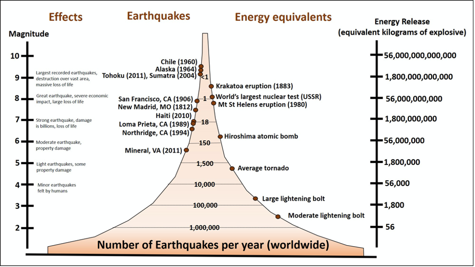
Another way to classify an earthquake is by the energy released during the event; this is referred to as the magnitude of the earthquake. Magnitude has been historically measured using the Richter scale; however, as the frequency of earthquake measurements around the world increased, seismologists realized the Richter magnitude scale was not valid for all earthquakes, specifically large magnitude earthquakes. A new scale called the Moment Magnitude Scale was developed, which maintains a similar logarithmic scale to the Richter scale. This scale estimates the total energy released by an earthquake and can be used to characterize earthquakes of all sizes throughout the world. The magnitude is based on the seismic moment, estimated based on ground motions recorded on a seismogram, which is a product of the distance a fault moved and the force required to move it. This scale works particularly well with larger earthquakes and has been adopted by the USGS.

Magnitude is based on a logarithmic scale, which means for each whole number increased, the amplitude of the ground motion recorded by a seismograph increases by 10 and the energy released increases by 101.5, rather than one. A magnitude 3 earthquake results in ten times the ground shaking as a magnitude 2 quake; a magnitude 4 quake has 102 or 100 times the level of ground shaking as a magnitude 2 quake, releasing 103 or 1000 times as much energy. For a rough comparison of magnitude scale to intensity (Table 6.3).

Table 6.3: Relationship between magnitude and intensity values.

Magnitude	Qualitative Descriptor	Typical Maximum Modified Mercalli Intensity
1.0 – 2.9	Micro	I– III
3.0 – 3.9	Minor	III - IV
4.0 – 4.9	Light	IV – V
5.0 – 5.9	Moderate	V – VI
6.0 – 6.9	Strong	VI – VII
7.0 -7.9	Major	VIII-VII
8.0 and above	Great	VII or higher

Why is it necessary to have more than one type of scale? The magnitude scale allows for worldwide characterization of any earthquake event, while the intensity scale does not. With an intensity scale, an IV in one location could be ranked II or III in another location, based off of building construction. For example, poorly constructed buildings will suffer more damage in the same magnitude earthquake as those built with stronger construction.

Energy comparison: On August 4th, 2020, 2,750 tons of ammonium nitrate ignited and exploded in the Port of Beirut in Lebanon. This explosion damaged most structures within a 3-mile radius and was heard in Cyprus more than 100 miles away. The explosion was devastating; hundreds were killed and thousands injured and many were displaced from their homes. This event was roughly equivalent to a 1-3 kiloton TNT explosion which roughly translates to a M4.5 earthquake. However, seismic stations throughout the region recorded the event as a M3.3. This discrepancy is likely due to the fact that the explosion was at the surface, resulting in most of the energy traveling up into the air and into the surrounding buildings in lieu of traveling through the rock.

Figure 6.12: Large earthquakes occur about once a year. Smaller earthquakes such as magnitude 2 earthquakes, occur several hundred times a day.

Figure 6.13: The P-waves are the first to arrive at each station, followed by the S-waves. The P-waves travel faster than S-waves the great distance between the two (S-P interval), the further away the earthquake epicenter.

 

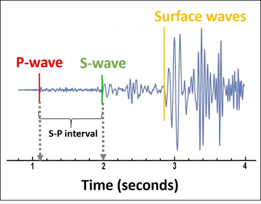
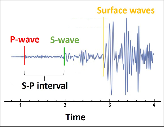
During an earthquake, seismic waves are propagated throughout the entire Earth. Though they may weaken with distance, seismographs are sensitive enough to detect these waves. In order to determine the location of an earthquake epicenter, seismographs from at least three different locations are needed. Once three seismographs have been located, the S-P interval must be measured (Figure 6.13). To do this, you must first determine when the P-wave arrived at the seismograph station. On the seismogram, find the arrival of the P-wave, which can be recognized by an increase in amplitude (wave height), and note the time of P-wave arrival. Repeat this procedure for the S-wave, then subtract the arrival time of the P-wave from the arrival time of the S-wave. In general, longer time S-P intervals indicate further station distance from an epicenter.

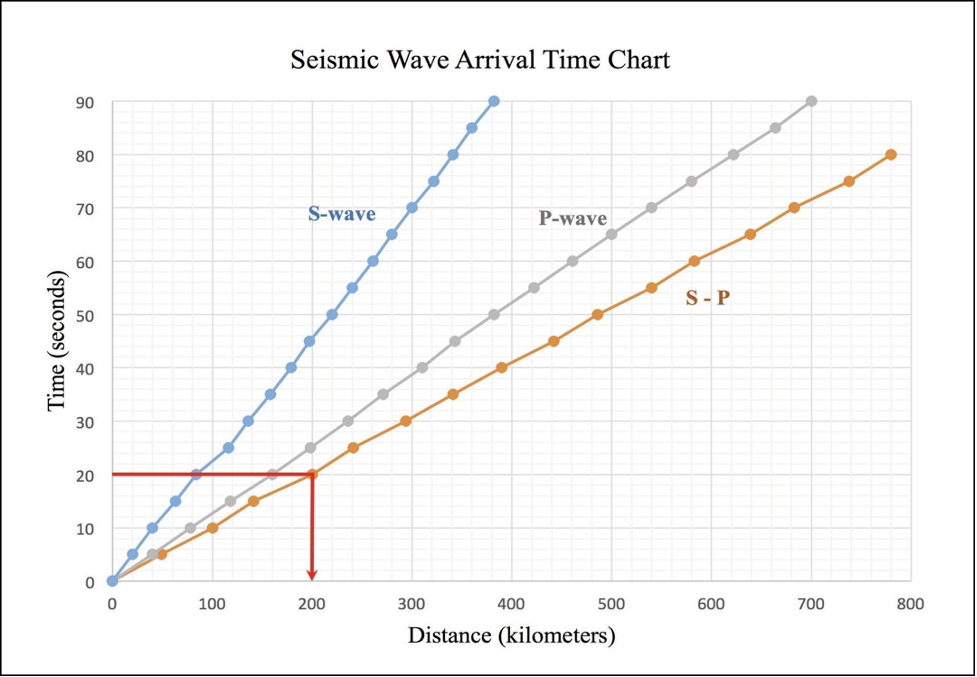
Once you have calculated the S-P interval, you will now be able to determine the distance to an earthquake epicenter from a specific seismic station. This is typically done using a travel-time curve, which is a graph of P- and S-wave arrival times (Figure 6.14).

Figure 6.14: A travel-time graph that includes the arrival of P-waves and S-waves. Note that these curves plot distance versus time and are calculated based on the spherical shape of Earth. Curves vary with the depth of earthquake because waves behave differently with depth and change in material. This curve is used for shallow earthquakes (<20 km deep) with stations within 800 km. The S-P curve refers to the difference in time between the arrival of the P-wave and S-wave.

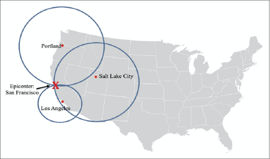
Though distance to the epicenter can be determined using a travel-time graph, direction cannot. To pinpoint the location of the epicenter, we can use distance information from three seismograph stations and triangulate. To do this, draw a circle around one of the seismograph locations with a radius of the distance to the earthquake. We know that the earthquake occurred somewhere along this circle, but a circle contains an infinite number of possible epicenters; this is why it is necessary to have data from at least three seismic stations. Draw a circle around at least two more seismograph locations, where the radius of each circle is equal to the distance from that station to the epicenter. The spot where those three circles intersect is the epicenter (Figure 6.15).

Figure 6.15: In order to locate this earthquake’s epicenter, seismograms from Portland, Salt Lake City, and Los Angeles were used. The time between P and S wave arrivals was calculated, and travel timetables gave a distance. Circles with each distance for their radii were drawn from each station. The one resulting overlap, at San Francisco, was the earthquake epicenter.

 

Hazards from Earthquakes

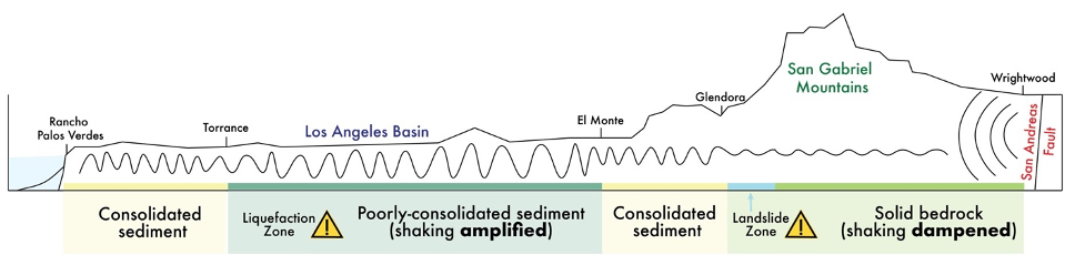
Earthquakes are among nature’s most destructive phenomena, and there are numerous hazards associated with them. Ground shaking can lead to falling structures, making it the most dangerous earthquake-related hazard. The intensity of ground shaking depends on several factors, including the size of the earthquake, the duration of shaking, the distance from the epicenter, and the material the ground is made of. Solid bedrock will not shake much during a quake, rendering it safer than other ground materials. Typically, seismic waves will amplify as they encounter weaker geologic materials (sediments), and this amplification can be destructive (Figure 6.16).

Figure 6.16: Earthquake waves amplify (wave height increases) in poorly consolidated sediments, which can lead to more intense shaking and liquefaction.

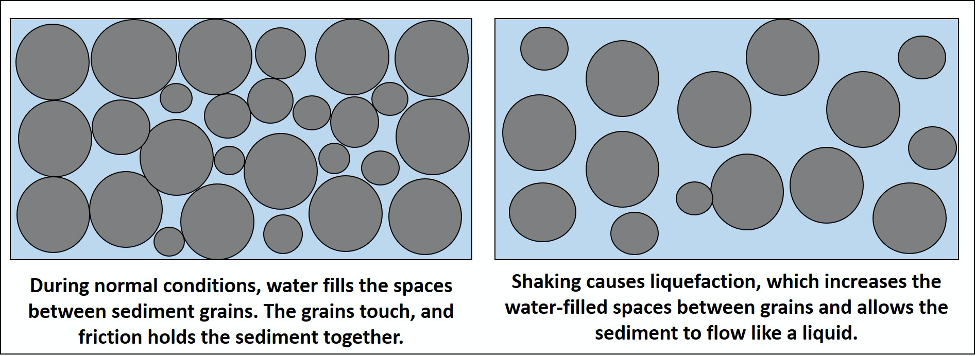
In addition to wave amplification, loose, water-saturated sediments or artificial fill can serve as sites for liquefaction. Normally, friction between grains holds them together; however, as unconsolidated sediments are shaken, water surrounds every grain, eliminating the friction and allowing them to liquefy (Figure 6.17). Liquefaction can cause major damage to buildings and infrastructure, sand and water to be ejected in “sand volcanoes”, and the ground surface to be permanently deformed. Want to see a fun experiment? Check out this jacuzzi filled with sand!

Figure 6.17: Left: During normal conditions, water fills the spaces between sediment grains. The grains touch, and friction holds the sediment together. Right: Shaking causes liquefaction, which increases the water-filled spaces between grains and allows the sediment to flow like a liquid.

Large (M7.5+) earthquakes typically displace the seafloor, which can trigger tsunamis. These large ocean waves are often associated with subduction zone earthquakes. The Sumatra-Andaman earthquake in 2004 triggered a tsunami in the Indian Ocean that resulted in almost 230,000 deaths. In 2011, the Tohoku earthquake off the coast of Japan triggered a tsunami wave that heavily impacted the country, killing more than 15,000 and causing the meltdown of the Fukushima Daiichi Nuclear Power Plant.

Figure 6.18: USGS geologists make measurements of fault rupture after the Searles Valley Earthquake, July 2019.

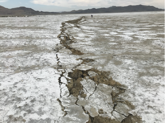
Earthquakes can also 1) ignite fires, like the conflagration experienced following the Great San Francisco Earthquake of 1906, 2) result in major ground rupture, like the rupturing experienced during the Ridgecrest earthquakes in 2019 (Figure 6.18), and 3) trigger landslides, like. the more than 10,000 landslides experienced in the LA area in the wake of the Northridge earthquake in 1994. Typically, landslides will occur in areas with steep slopes, like the mountains, or underwater. Underwater landslides may also trigger tsunami, and, if coupled with a subduction zone earthquake, may result in a taller-than-predicted wave. Earthquake-prone areas can take steps to minimize destruction, such as implementing strong building codes, early warning systems, addressing poverty and social vulnerability, retrofitting existing buildings, and limiting development in hazardous zones. Earthquake forecasting (Figure 6.19) can help communities plan for their future risk. Want to know your hazard potential? Visit the California Department of Conservation’s EQ Zapp: California Earthquake Hazards Zone Application.

Figure 6.19: USGS map showing (1) the locations of major populations and (2) the intensity of potential earthquake ground shaking that has a 2% chance of occurring in 50 years.

Induced Seismicity

In some intraplate areas of the country, like Oklahoma, earthquake numbers in a single year can exceed even what we experience here in California. The majority of these earthquakes are a result of human activity and are known as induced seismicity. Humans have induced earthquakes in the past, but the increasing frequency of episodes of induced seismicity has led to more dedicated research into the problem. Evidence points to several contributing factors, all related to types of fluid injection used by the oil industry. Hydraulic fracturing, also referred to as fracking, has been used for decades by oil and gas companies to improve well production. Fluids, usually water, are injected at high pressure into low-permeability rocks to fracture the rock. As more fractures open within the rock, fluid flow is enhanced and more distant fluids can be accessed, increasing the production of a well. In the past, this practice was utilized in vertical wells. However, with the recent advent of horizontal drilling technology, the fracking industry has really taken off. Drillers can now access thin horizontal oil and gas reservoirs over long distances, greatly increasing well production in rocks that formerly were not exploited, driving a boom in US natural gas and oil production.

While there have been many reports in the media that blame the process of hydraulic fracturing for all the increased seismicity rates, this is not the full story. Fracking mainly produces very minor earthquakes, less than magnitude 3 (although it has been shown to produce significant earthquakes on occasion). Instead, the majority of induced earthquakes are actually caused by the injection of wastewater deep underground. Wastewater injection is a byproduct of fracking, so ultimately the industry is to blame. As wells are developed (by fracking or other processes), large amounts of waste fluid, which typically contain potentially hazardous proprietary chemicals, are created. When the fluids cannot be recycled or stored in retention ponds above ground, they are injected deep underground, theoretically deep enough to not encounter oil reservoirs or water supplies. These wastewater wells are quite common and are considered a safe option for wastewater disposal. By injecting this water in areas that contain faults, however, the stress conditions on the faults change as friction is reduced, which can result in movement along faults and earthquakes.

In 2005, the White Wolf fault located southeast of Bakersfield (Figure 6.20), experienced an earthquake swarm. Peak activity occurred on September 22, 2005 with multiple quakes ranging from M4.3-4.6. Nearby is the Tejon Oil field, which between 2001 and 2010 increased the rate of wastewater injection by over 26.4 million gallons of water each month. Ultimately, this put pressure on the White Wolf fault, which then ruptured, producing the swarm. Want to learn more about fracking? Visit the USGS Myths and Misconceptions About Induced Earthquakes.

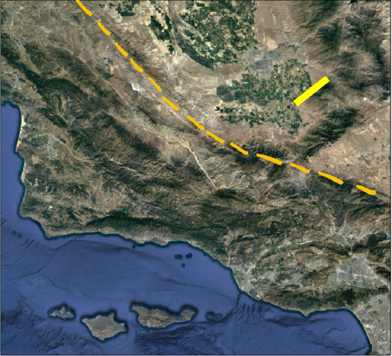
Figure 6.20: White Wolf Fault shown in yellow with the San Andreas Fault in orange.

Attributions

• Figure 6.1: “2019 Ridgecrest Earthquake” (Public Domain; USGS)

• Figure 6.2: “Earthquake Hazard Map” (Public Domain; USGS)

• Figure 6.3: “Seismic Waves” (CC-BY-NC 2.5; xkcd via xkcd.com)

• Figure 6.4: “Earthquake Focus and Epicenter” (CC-BY 4.0; Chloe Branciforte, own work)

• Figure 6.5: “Wadati-Benioff Zone” (CC-BY 4.0; Chloe Branciforte, own work)

• Figure 6.6: Derivative of “P wave” (Public Domain; USGS)

• Figure 6.7: Derivative of “S wave” (Public Domain; USGS)

• Figure 6.8: Derivative of “Surface Wave Motion” (CC-BY 3.0; Jcrane81 via Wikimedia Commons) by Chloe Branciforte

• Table 6.1: “Seismic Waves” (CC-BY 4.0; Chloe Branciforte, own work)

• Figure 6.9: “USGS Seismograph Point Reyes” (CC-BY-SA 3.0; Dvortygirl via Wikimedia Commons)

• Figure 6.10: Derivative of “S-P Interval Seismogram Distance to Earthquake” (CC-BY-SA 4.0; Benjamin J. Burger via Wikimedia Commons)

• Table 6.2: “Modified Mercalli Intensity Scale” (CC-BY 4.0; Chloe Branciforte, own work)

• Figure 6.11: “ShakeMap for 2019 Ridgecrest Earthquake” (Public Domain; USGS)

• Table 6.3: “Magnitude and Intensity” (CC-BY 4.0; Chloe Branciforte, own work)

• Figure 6.12: How Often Do Earthquakes Occur? ©IRIS Consortium. Adapted and used with permission (16 November 2020). [All rights reserved].

• Figure 6.13: Derivative of “S-P Interval” (CC-BY-SA 4.0; Benjamin J. Burger via Wikimedia Commons) by Chloe Branciforte

• Figure 6.14: “Seismic Wave Arrival Chart” (CC-BY-SA 3.0; Randa Harris, own work via LibreTexts)

• Figure 6.15: “Epicenter Distance” (CC-BY-SA 3.0; Randa Harris, own work via LibreTexts)

• Figure 6.16: “Liquefaction and Amplification in SoCal” (CC-BY 4.0; Emily Haddad, own work)

• Figure 6.17: “Liquefaction” (CC-BY 4.0; Chloe Branciforte, own work)

• Figure 6.18: “Surface Rupture” (Public Domain; USGS)

• Figure 6.19: “USGS Earthquake Hazard Map” (Public Domain; USGS)

• Figure 6.20: “White Wolf Fault” (CC-BY 4.0, Chloe Branciforte via Google Earth, own work)