
2.5: Lab 5 - More about Folds
- Page ID
- 12511

Multiple planes on the stereographic projection
The techniques you used in the last lab work well for folds that are perfectly cylindrical, and where the orientations of the folded surfaces are known with great precision. However, in many cases, folded surfaces are not perfectly cylindrical, and small variations in dip, and measurement errors, mean that the geometry is not perfect. Under these circumstances, to determine the orientation of a mean fold axis, it is desirable to measure a large number of orientations, and to use a statistical approach.
Unfortunately, plotting large numbers of great circles rapidly produces a very cluttered projection. For this reason, it is much better to plot poles to the folded surfaces rather than great circles. In the ideal case the poles should all lie in the profile plane, and therefore they will plot as points on a single great circle. In real life, things are not so simple; the poles appear scattered in a band, or girdle, on either side of the profile plane, which has to be estimated as a ‘best-fit’ great circle through the densest band of points.
There is an additional problem, however. If you look at the Wulff net, you will see that the 2° and 10° squares project much larger near the primitive than they do at the centre of the net. This means that plots made with the Wulff net should never be used for statistical inferences based on density of points, because it artifically increases the density in the centre and decreases it on the primitive.
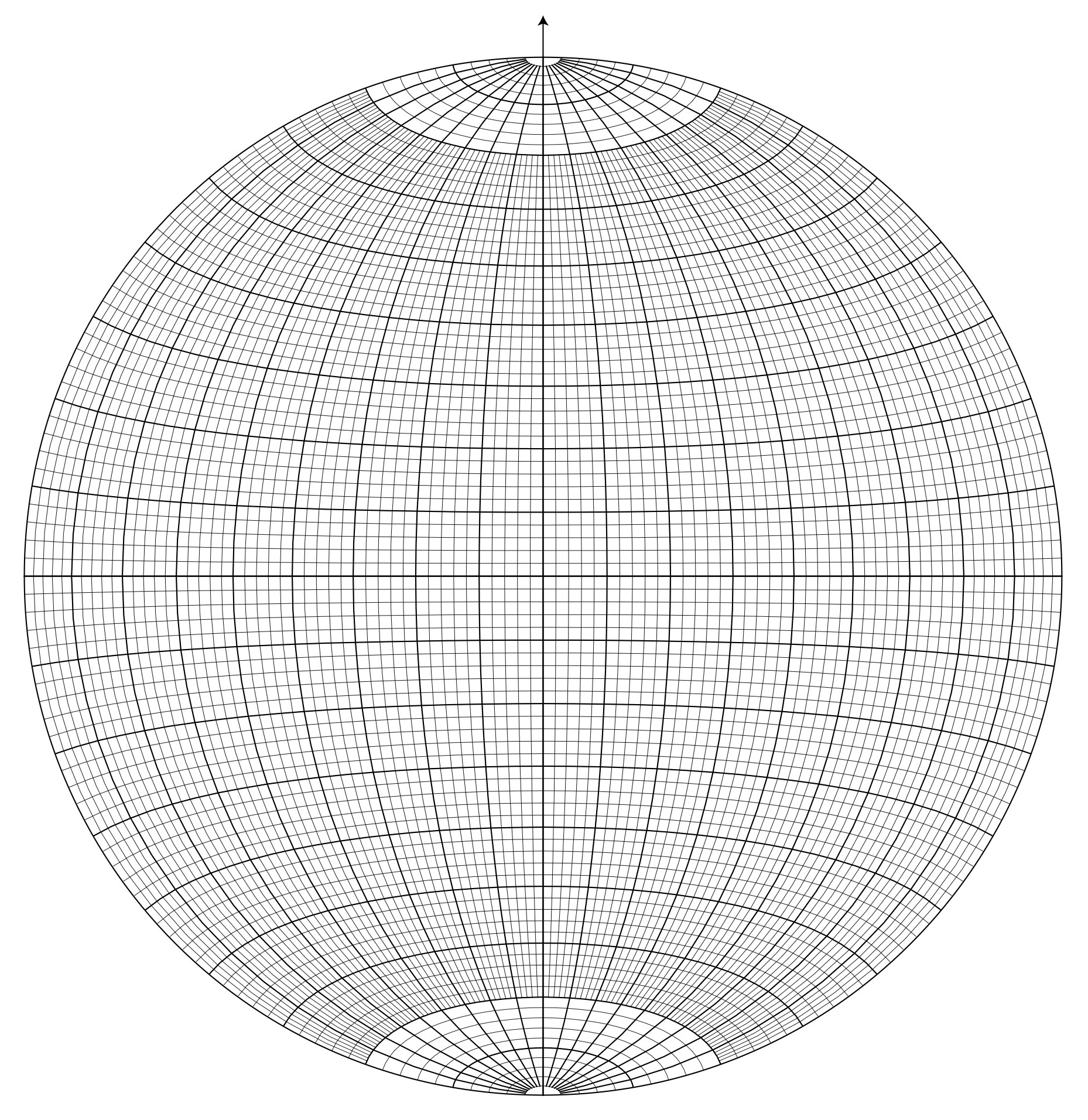
For this reason, a modified stereographic projection, called the equal area projection is used, based on the Schmidt net. All the operations you have met so far are the same on the two nets; the only difference is that the equal area projection does not preserve circular arcs – the great and small circles are complex curves and cannot be drawn with a compass. For this course make sure your net is printed so that its diameter is exactly 15 cm.
Pi diagram
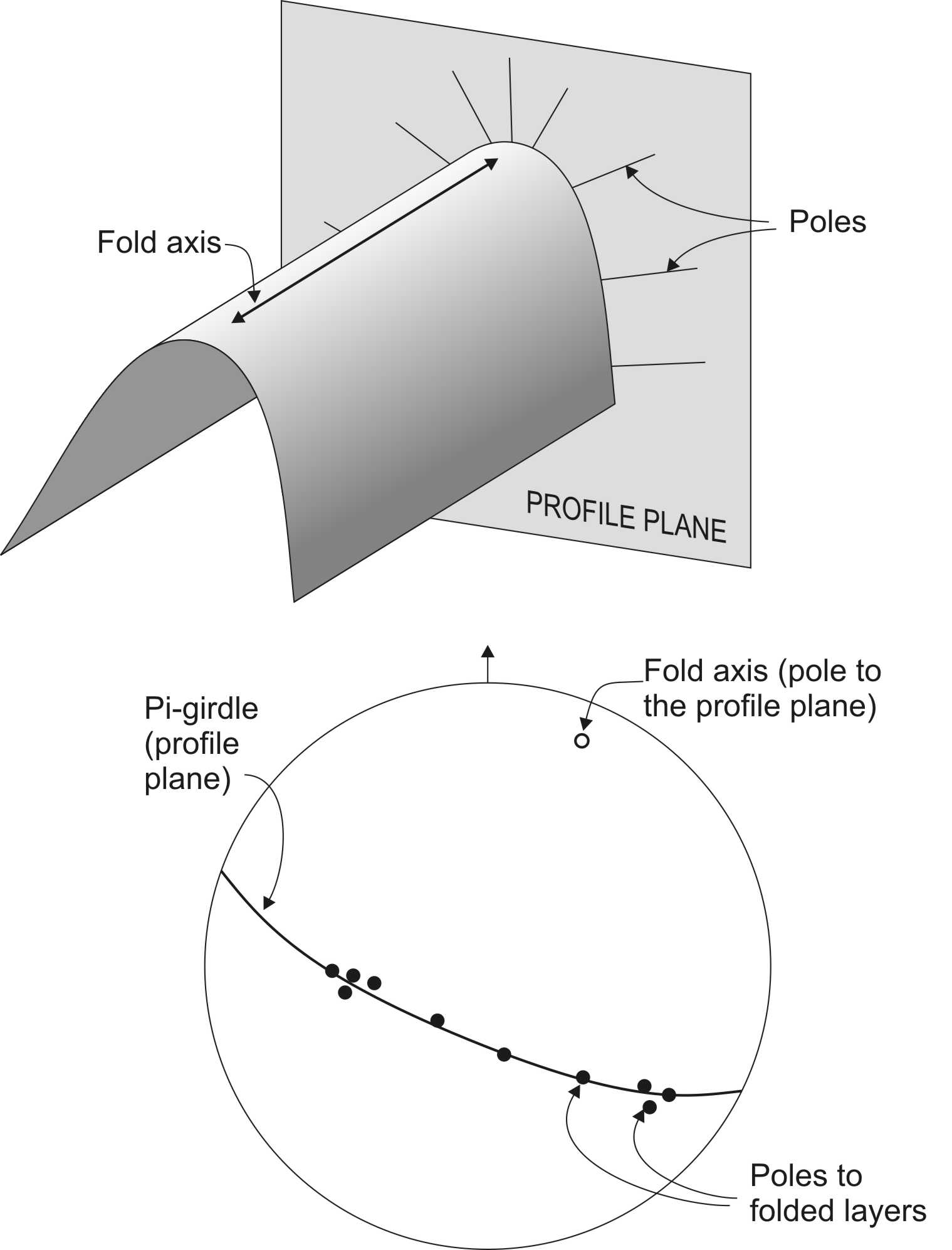
The resulting plot of poles to planes on a equal area projection is called the pi-diagram, which is the most common method used to find the mean fold axis in an area of folded rocks where, as often happens, individual fold hinges are not exposed. The principle of the pi-diagram is illustrated in Figure 1. In a cylindrical fold, the poles to the folded layers are lines perpendicular to the fold axis. They therefore lie in the profile plane, the plane that is perpendicular to the fold axis. If the folds are not perfectly cylindrical, or if there are small errors in the measurements, the lines will not lie precisely in the profile plane, but will be close to it.
Contours on the axial surface
Maps of areas with folded rocks can be challenging because of the number of surfaces involved, and because of rapid changes of strike and dip. Often, even though layers may show complex folding, axial surfaces may be approximately planar. Under these circumstances it makes sense to separate the limbs of the fold by drawing axial traces, and even to draw contours on the fold axial surfaces. When doing this, it’s important to remember that a single fold will have multiple hinges (one for each folded surface), but that these hinges lie in a single fold axial surface.
Assignment
1.* The area you contoured last week (Great Cavern petroleum prospect) shows strike and dip symbols representing measurements of bedding orientation.
Plot poles to bedding for all the strike and dip measurements on an equal area projection, to make a pi-diagram. Find and draw the best-fit great circle through the poles; this represents the profile plane. Mark the best estimate of the fold axis (pole to the profile plane) and determine its trend and plunge. Is it similar to the value you obtained by contouring last week, and to the values obtained by your other team members?
2.* Look at the map of Somerset County in the Appalachians of Pennsylvania. The area has a long history of coal mining, and a number of coal seams are identified on the stratigraphic column that doubles as a legend.
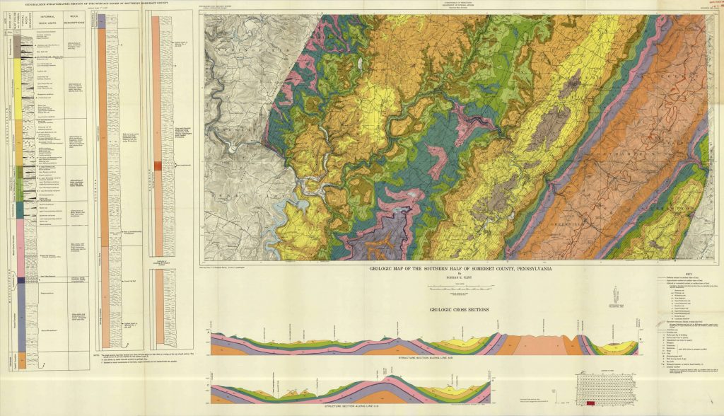
a) The map has structure contours, shown in red, drawn on one surface. Which one surface? (Note: each formation on the map has a top and a bottom surface, so just a formation name is not a complete answer; your answer should be in the form ‘the boundary between Formation x and Formation y’.)
b) Use the spacing of the structure contours to determine the strike and dip, at its steepest point, on each limb of the most conspicuous fold. Note that the contours are in feet, and the scale of the map is 1:62500 (about 1 inch to 1 mile). Make sure that in your dip calculation you use the same units vertically and horizontally. Use the points where the contours cross the fold hinge to determine the average trend and plunge of the fold hinge.
c) Plot both limbs of the fold from part ‘b’ on a stereographic projection. Using the intersection and the angle between the planes, estimate the plunge and trend of the fold axis, and the interlimb angle of the fold.
d) Based on these observations, describe the orientation (plunge, tightness, overall orientation) of the fold in words (e.g. ‘tight, steeply plunging synformal anticline’)
e) If the fold is cylindrical, the fold axis orientation determined stereographically should coincide with the hinge orientation determined by contours. How close are they (in degrees)?
3. Map 1 contains an angular fold in a more general orientation than the perfectly horizontal folds you dealt with last week. In addition there are some unfolded rocks and an intrusion. An unconformity separates the more highly deformed folded rocks from the gently dipping younger rocks. To help you solve the map, note that in the west of the map, the bedding traces are somewhat parallel to the topographic contours. These regions correspond to a gentle fold limb. Elsewhere, the geological boundaries cut across the contours at a steeper angle; this is a steep fold limb. Fold hinges can also be identified on the map from sharp swings in the trace of bedding that are not obviously related to valleys and ridges. Before you begin, try to use these hinges to sketch where there might be fold axial traces; these should separate regions of steeper and more gently dipping beds. Do this very lightly – it is likely you will change your mind as you proceed.
a) Identify the various surfaces on the map. First, mark the unconformity surface in green or yellow. Then mark the boundary between marble and amphibolite in blue or violet. Mark the boundary between amphibolite and schist in red or orange. (Note: the colour scheme is provided for convenience. If you choose different colours, you must use them consistently throughout this exercise.)
b) Draw structure contours on the green surface.
c) Draw structure contours on the red surface. You will find that there are two parts to this surface: a steep limb and a gentle limb. These have separate sets of contours. The two sets of red contours intersect in a fold hinge. Mark this on the map and trace over it with red.
d) Repeat for the blue surface and mark the blue hinge.
e) The red hinge and the blue hinge are both lines that lie in the axial surface of the fold. Join points of equivalent elevation on the red hinge and blue hinge with lines: these are structure contours on the axial surface. Number them in purple or violet.
f) Use the axial trace contours to predict the outcrop trace of the axial surface, and draw this trace on the map. The axial trace should separate the steep limb from the gentle limb of the fold.
g) Make a cross section along the line XY.
h) Plot both fold limbs, the axial surface, and the unconformity as great circles on an equal area projection. Mark the point corresponding to the orientation of the fold axis.
i) Describe the orientation of the fold in words as completely as you can
j) List the events in the geological history of the area for which you have evidence, starting with the oldest. In the case of the three folded units, where there is no direct evidence of age, you should assume that the fold is upward facing (i.e. synforms are also synclines; antiforms are also anticlines).