1.11: Faults
- Page ID
- 12519


Introduction
Fractures are known as faults if there has been significant displacement of one side relative to the other, parallel to the fracture plane. Faults have had enormous economic impact in the exploration for natural resources. Faults affect the flow of fluids in the Earth’s crust, and thereby control the distribution of water, oil and natural gas. Fractured material along a fault plane may form a porous breccia (pronounced “bretchya”). Fluid passing through breccia may deposit valuable minerals. Faults are also important to humans because they generate earthquakes.
An extensive terminology has developed around faults, their geometry, and movement (kinematics). It is important to distinguish between descriptive (geometric) terms, which tell us about the orientation of a fault and the offset of layers on either side, and kinematic terms, which describe the distance and direction of fault movement.
Faults, fault zones, and shear zones
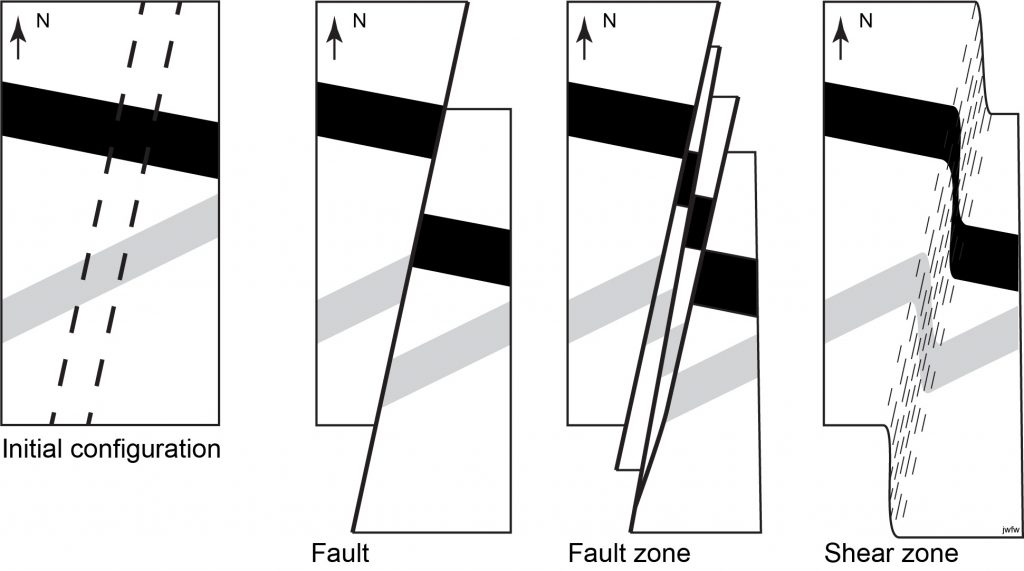
Strictly speaking, a fault is a single fracture surface. However, many mapped faults turn out to have multiple fault strands, all roughly parallel, but branching and joining (“anastomosing”) along their strike. This type of fault array is called a fault zone. The total offset of the fault zone is distributed across the zone. Each fault in the zone offsets the rocks on either side by a small amount. These add up across the fault zone to a much larger offset.
A related structure is a shear zone. A shear zone is the ductile equivalent of a fault zone – a belt of rock across which movement has caused a significant amount of offset between the two sides. However, a shear zone is a ductile structure, typically formed at depth where the deformation of the mineral grains is plastic, not brittle. The movement in a shear zone is distributed across the zone, rather than being restricted to discrete brittle faults. It is likely that most faults that deform the upper crust pass at depth into shear zones in the lower crust.
At [pb_glossary id=”779″]map scale[/pb_glossary], faults and shear zones look the same – a line across which older structures are offset. At outcrop (mesoscopic) or microscopic scale they look rather different.
The orientation of natural faults often varies and they eventually disappear along strike; however, they do tend to have surfaces that are more planar than other types of geological surfaces, at least over distances of a few kilometres. Faults can be recognized at a variety of scales from centimetre-scale offsets in an individual outcrop to faults that can be traced on the ground for tens to hundreds of kilometres such as the San Andreas Fault.
Fault geometry
Strike and dip
A fault is a planar geologic structure. Like any planar structure, it has an orientation that may be characterized by strike and dip. For small faults, it may be possible to walk up to an outcrop and measure the orientation with a clinometer. Large faults tend to be poorly exposed, because rocks close to the fault plane are fractured and broken, and therefore are easily weathered. For large faults, the orientation may be more easily determined by drawing structure contours. If the fault is planar, the strike and dip will be constant, and the structure contours will be parallel, straight, and equally spaced. If the fault is curved, then structure contours may show changes in orientation and spacing.
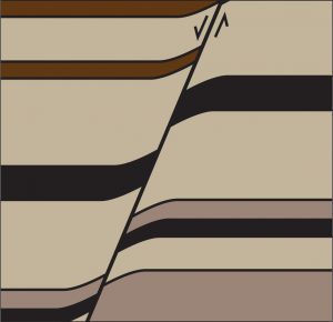
The blocks of rock on either side of a fault plane are the walls of the fault. If a fault has a dip (other than 90°) then one wall overhangs the other. For example, if a fault dips east, then the east wall must overhang the west wall. The wall located on the down-dip side of the fault is called the hanging wall. The wall located to the up-dip side of the fault is called the footwall.
If these are not clear, think of a geologist standing in a small cave exactly on a fault plane that dips moderately. The geologist’s feet will rest naturally on the footwall, while the hanging wall will overhang the geologist’s head.
If a fault is vertical, it is not possible to characterize a footwall and a hanging wall. Under those circumstances it is better to use compass directions to identify the walls: e.g. “east wall”.
Offset and separation
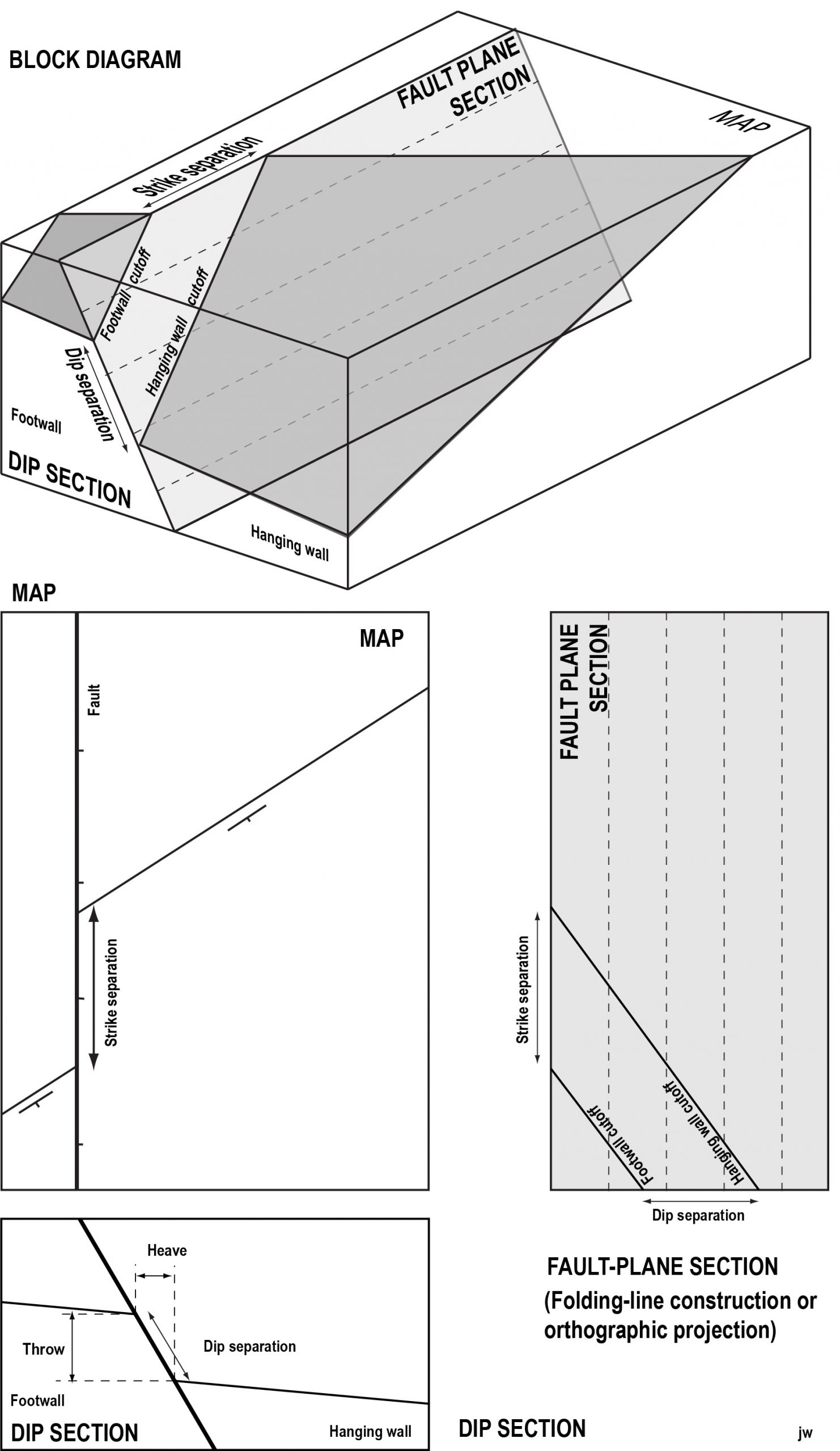
If a fracture is a fault, there will also be offsets of beds or other older surfaces that are cut. On a map or cross-section, the points where the trace of a fault cuts the trace of an older surface are called cutoff points (or cut-off points). In three dimensions, the lines where a fault intersects an older surface are called cutofflines (Fig. 3). The distance between the two cutoff lines, for a given surface, is called the separation of the surface. In plan view, as seen on a map of a horizontal surface, the distance of offset measured parallel to the strike of the fault is called the strike separation. The strike separation can be sinistral (also known as left-lateral) or it can be dextral (also known as right-lateral). In cross-section view, parallel to the dip of the fault, the separation is called dip separation. If the beds in the hanging wall are offset below those in the footwall the separation is normal. If the beds in the hanging wall are offset above those in the footwall then the separation is reverse. The vertical and horizontal components of dip separation were very important in old mining operations, and are known as throw and heave respectively.
It’s important to realize that these measurements of separation are geometric. They tell you little about kinematics. In the diagram below, the arrows on the fault plane show that an infinite number of slip directions is compatible with a given fault separation.
One feature that may be recognized in the field and is a common result of relatively recent fault activity is the development of a fault scarp, which is that part of the failure surface exposed by movement of the rock masses. In studies of recent faults (neotectonics) the fault scarp may give an indication of separation.
However, over time the high-standing block tends to be levelled by erosion. The surface expression of the scarp is subdued or eliminated and may be of little help in locating ancient faults. Where fault scarps do occur along ancient faults, the direction of slope tends to be determined by which side has the more erosion-resistant rocks, not by the sense of separation on the fault. In fact, locating faults in Precambrian terrains may be quite difficult because rocks affected by faulting tend to be easily eroded. Such faults often occur in low-lying regions occupied by swamps, streams or heavy vegetation.
Fault kinematics: measuring slip
Slip
The slip is a line that lies in the fault plane; slip represents the distance and direction of movement between the two blocks of rock on either side of the fault. The slip is a vector – it has a distance and direction. The direction of slip may be specified by trend and plunge, or by rake within the fault plane. When the rake of the slip is close to the strike of the fault, the fault is called a strike-slip fault. When the rake is near 90°, close to the dip of the fault, the fault is a dip slip fault.


It is important to understand that slip cannot be determined from the separation of a single offset surface; we need additional information such as slickenlines (scratches or fibres on the fault surface) to give us the direction of the slip. Figure 3 illustrates the problem: multiple slip vectors would be consistent with the separations shown by the fault.
Piercing points
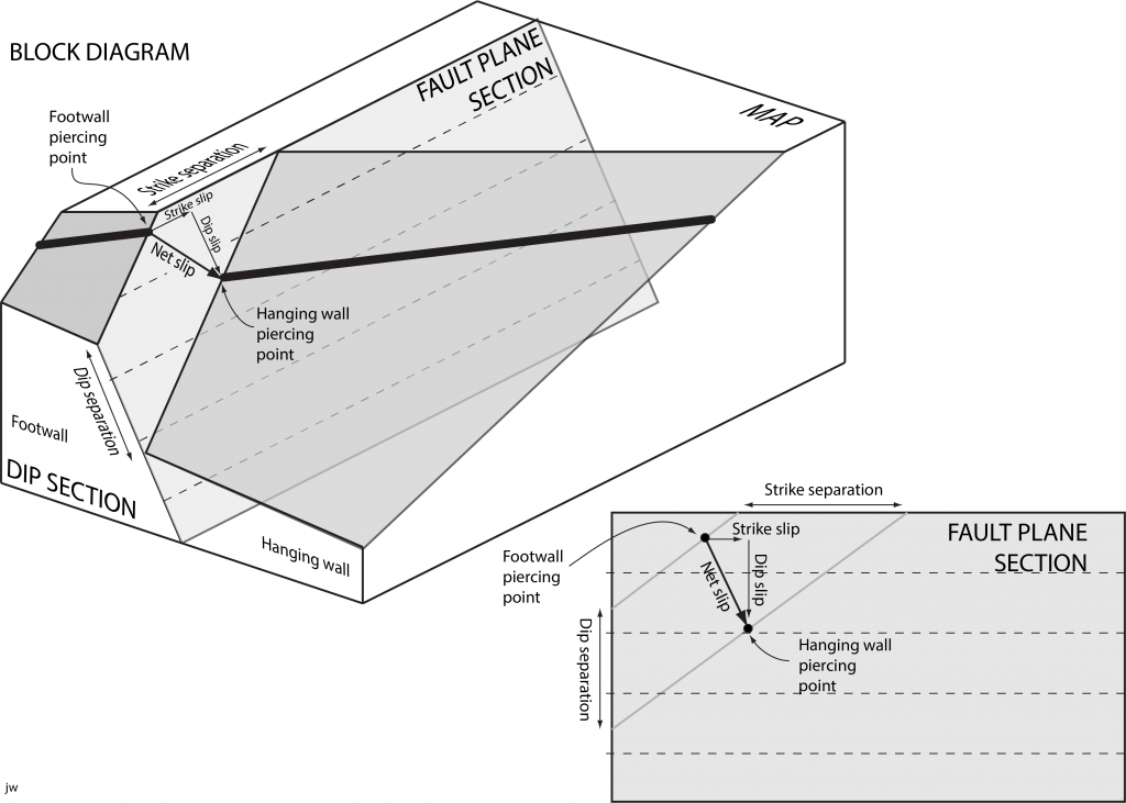
If we have a line that is cut and displaced by the fault, we can solve uniquely for the slip vector. The intersection of a line with a fault plane produces a point, called a piercing point. If we can locate the piercing points for the blocks on either side of the fault then we will be able to determine the displacement vector as shown in Figure 5.
The slip is a line that lies in the fault plane, that represents the distance and direction of movement between the two blocks of rock on either side of the fault. The slip is a vector – it has a distance and direction. The direction of slip may be specified by trend and plunge, or by rake within the fault plane. When the rake of the slip is close to the strike of the fault, the fault is called a strike-slip fault. When the rake is near 90°, close to the dip of the fault, the fault is a dip-slip fault.
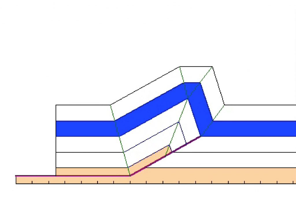
The question is, what will we use for a line cut by the fault? Recall that two non-parallel planes intersect along a line, and you have your clue. If two planar features (such as veins, unconformities, formation boundaries, or igneous dykes) intersect each other, then their line of intersection may in turn pierce the fault plane. Figure 6 shows an example where an igneous intrusion is truncated by an unconformity at a subcrop line. Displacement along the fault offsets the subcrop line producing piercing points for hanging wall and footwall. A unique vector joins the piercing points, characterizing the fault displacement.

Fold hinges also make excellent piercing points. Figure 7 shows an example.
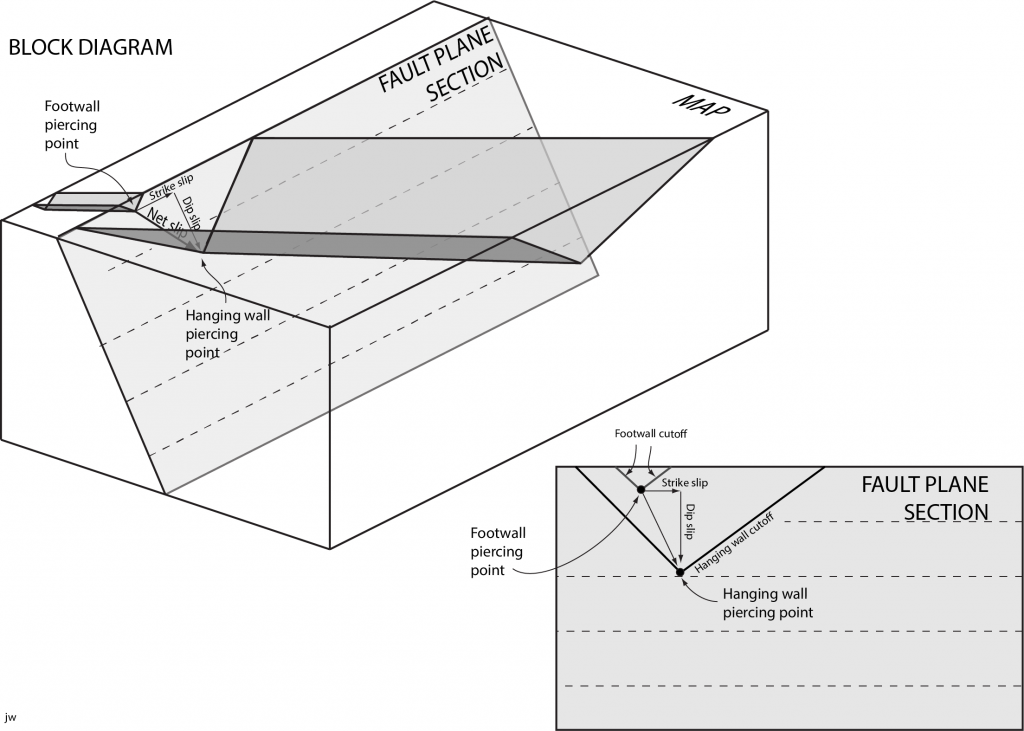
Figure 8 shows a second circumstance in which the net slip can be calculated. In this example, striations on the fault surface (known as slickenlines) allow the direction of slip to be determined. It is then possible to construct artificial piercing points on cutoff lines at opposite ends of a single slickenline. The amount of slip can be measured between the constructed piercing points.

Components of slip
Once the net slip vector is known, it can be broken down into components. The component of slip parallel to the strike of the fault is the strike slip. The strike slip may be characterized as sinistral (or left-lateral) or dextral (right-lateral). The component parallel to the dip of the fault is called the dip slip. The dip slip may be characterized as normal or reverse, depending on whether the hanging wall moved up or down relative to the footwall. If the dip slip is much larger than the strike slip, then the fault is a dip-slip fault; the rake of the slip in the fault plane is close to 90°. If the strike slip is much greater, then the fault is a strike-slip fault; the rake of the slip is close to zero or 180°. If the dip slip and strike slip are of comparable magnitudes, then the fault is an oblique-slip fault.
Fault-plane sections
Most calculations involving fault slip are best carried out on a cross-section that lies in the fault plane. Figures 3, 5, 6, and 7 are each illustrated with a diagram showing a fault-plane cross-section. Most of the significant measurements of separation and slip can be made directly on the fault-plane cross-section. Of course, in general such a cross-section will not be vertical. Special techniques are necessary for the construction of non-vertical cross-sections. A plan view of a dipping geological surface is sometimes called an orthographic projection (because features are projected perpendicular to the surface onto a plane sheet of paper) and sometimes called a folding line construction (because we treat the sloping fault plane as if we have folded it around one of its structure contours until it is in the horizontal plane of a table top.) Typically, we begin by placing a sheet of paper with its edge along one of the structure contours on the fault plane. This line becomes the folding line. Next, we use a stereographic projection or contours to determine the rake of various lines on the fault surface and draw them in.
Sometimes it also helps to draw the projected structure contours as horizontal lines on a fault-plane section, to show elevations above sea level (see fault-plane sections in Figures 3, 5, 6, and 7). The lines are not spaced as they would be on a vertical cross section. If the contour interval is i and the fault plane has dip d, the spacing of the contours on the fault plane section will be:
i’ = i / sin(d)
Features of faults in the field
In the description of individual faults, it is generally possible to distinguish a core zone from a surrounding damage zone.
In the core, the rock has been broken up and moved around by fault movement so that the original pieces are separated from their neighbours. In the core zone it is no longer possible to see how the original pieces for faulted rock were fitted together.
In the damage zone, the rocks are fractured and may show other deformation features such as folds. However, the movement is not so great as to obliterate earlier structures, and it is at least possible to see how the pieces of damaged rock can be fitted back together.
Fault rocks: fault core
Several names are given to fragmented and other rocks of the fault core.
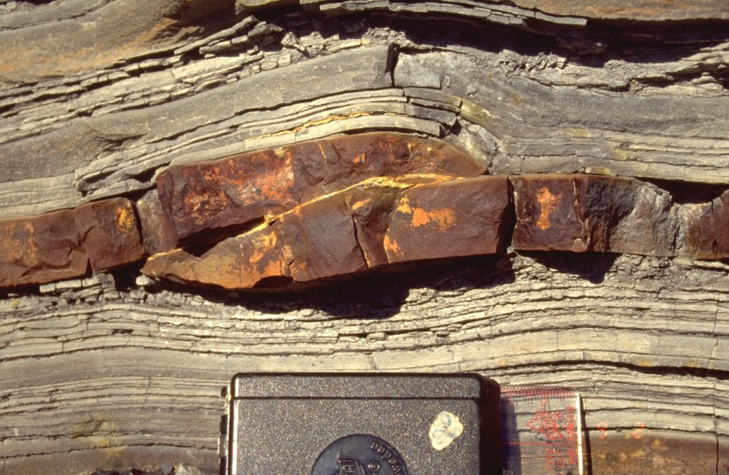
Breccia is a rock composed of typically angular fragments of the walls of the fault that have been rotated and moved out of their original positions. The fragments in a fault breccia may be huge, or may range down to about 2 mm. The term microbreccia may be used for a fine-grained breccia. Although the grain-size limits for breccia and microbreccia are not precisely standardized, it is reasonable to use microbreccia for fragments that are 2-4 mm in diameter (by analogy with the grain size of microconglomerate in sedimentary petrology).
Cataclasite is fragmented material that is sand-size or smaller. Note that neither breccia nor cataclasite typically has a fabric – the fragments are randomly oriented.
Gouge is the name given to clay-rich fault material, typically produced from faulting of fine-grained sediments. Because clay can behave in a ductile manner even under near-surface conditions, gouge can develop some fabric, because the clay particles become smeared into an orientation parallel to the fault plane. Gouge is typically very soft in outcrop. In the subsurface, gouge is very important, as a thick gouge layer may make a fault plane impermeable to fluids, whereas breccia and cataclasite are typically permeable.
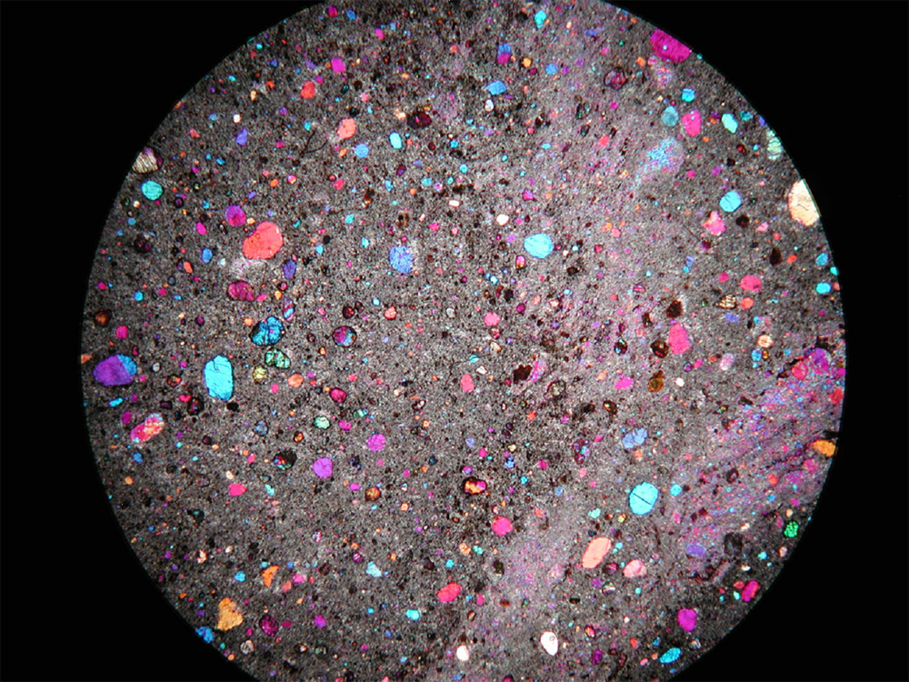
[Note on mylonite: Mylonite is a name given to fine-grained rock that has formed through ductile shearing and recrystallization in a shear zone. Mylonite is distinguished from breccia and cataclasite because it has a strong metamorphic fabric and often shows spectacular crystallographic preferred orientation – CPO – when viewed under the microscope in thin section. Confusion arises because when mylonite was first described in the 19th century, it was thought that the fine grain size resulted from brittle fracturing – the word ‘mylonite’ is derived from a Greek word for milling flour. In the 20th century the study of metals in industrial processes showed that ductile deformation could lead to the grain-size reduction seen in mylonites]
Pseudotachylite is material that was melted by heating during fault movement. Pseudotachylite is typically dark and very fine-grained or glassy. It may occur in small dykelets that penetrate the wall rock of the fault. Pseudotachylite takes its name from an old term for a very fluid igneous lava, tachylite. Pseudo-tachylite looked the same but had a very different origin.
Deformation adjacent to faults
Riedel shears are small shears that develop in response to stresses in the fault walls during fault propagation and movement. Synthetic Riedel shears, or R-shears, have an orientation at about 15° to the main fault plane, and display the same sense of shear as the main fault, as shown in Fig. 10. Less commonly, antithetic Riedel shears, or R'-shears, are also developed, at about 75° to the fault plane. These have a sense of shear opposite to that of the main fault. The synthetic and antithetic shears form a conjugate set, and therefore can be used to indicate the orientation of the stress axes when they formed.

Fault-bend folds. If a fault is curved, movement of the fault inevitably causes bending of either the hanging wall or the footwall or both. (If this did not happen, caverns would open up within the Earth as faults moved; lithostatic pressure prevents this from happening.) Fault-bend folds are particularly common in thrust belts like the Canadian Rocky Mountains.
Detachment folds. Sometimes, the amount of slip on a fault varies across the fault surface. Some sections have moved more than others. At the boundary between the sections, deformation in the wall rocks becomes intense, sometimes leading to the formation of detachment folds.

Drag folds. Sometimes, a fault will ‘lock’ during its development, and if this happens deformation may be spread through the wall rocks. If conditions are right, this deformation may be ductile and features in the wall rocks may be bent so that they become folded. Such folds are called drag folds. Drag folds can closely mimic fault propagation folds (below) that are formed at the tip of a fault as it develops. Many folds formerly categorized as drag folds are now interpreted as fault-propagation folds.
Fault-propagation folds form as faults develop, and combine some of the features of fault-bend and detachment folds. As a fault develops there will be a fault tip at the point separating slipped rock from rock that has not yet slipped. Fault-propagation folds form at this fault tip, and shorten one wall of the fault relative to the other. They are also common in thrust belts like the Rockies.