3.4: Stream Networks, Drainage Basins, and Divides

3.4.1 Tracing Stream Courses

In most areas of the world, except in the driest of deserts (and beneath glaciers), one can trace fairly easily on a topographic map the system of main streams and their tributaries. In some places streams “expand” into lakes, but the principle is the same.

Permanent streams are always shown as thin blue lines on official topographic maps, and ephemeral streams (those that flow only after a heavy rain) are often shown as dot–dash blue lines. Many well-defined valleys, however, which presumably would have streams flowing in them briefly after a heavy rain, have no streams shown in them. These are usually located in the headwaters of larger streams, which are shown on the map. So it’s just a matter of extending the streams shown on the map farther upstream, to where valleys are no longer defined and the land surfaces slopes uniformly. (Remember about the “V”s of the contour lines pointing upstream in valleys.) You yourself can trace the courses of such streams by recognizing the position and downslope direction of such valleys.

Here are some points that should help you in tracing stream courses where there are valleys with no stream shown in them.

1. Keep firmly in mind that in a valley, the contours tend to “vee” up the valley. You know that’s happening by seeing that the “vees” point in the direction of increasingly high contour lines.
2. When you draw the stream course, make it pass directly through the crotch of each contour “vee”. Streams tend to be curvy in real life, so don’t hesitate to end up with a curvy stream.
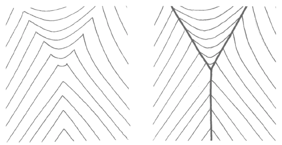
3. You are likely to find places where two tributary streams come together, at what’s called a confluence, to form a main stream. With a margin of error of the space of one contour interval, it’s easy to locate such a confluence: just look for places where a contour with one “vee” is succeeded upward by a contour with two closely spaced “vees” (Figure 1-44). The confluence lies somewhere between those two contours.

Figure 3-44. How you can locate the point of stream confluence by examining the “V”s of the contour lines.

3.4.2 Stream Divides and Drainage Basins

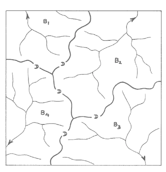
It should make sense to you that the land area between individual streams is on at least slightly higher ground than the streams themselves; if not, then the whole area would be a lake. (The exception to that last statement, fairly common in New England, involves low-lying wetlands bordered by or laced with well-defined streams.) Somewhere on that higher ground is a stream divide: a continuously curving locus of points on the map separating an area of the land surface with drainage into one stream from an area of the land surface with drainage into another stream (Figure 3-45).

Stream divides partition a given area of the land surface into drainage basins, each drained by a different main stream and its various tributary streams (Figure 3-45). Except in unusual situations, the land area is partitioned exhaustively and non-overlappingly into drainage basins.

If you are dealing with a fairly small area of the land surface, as represented, for example, by a 7-1/2' topographic map, you run into the uncertainty about whether a stream that runs off the edge of your map, along with its drainage basin, runs into one of the other streams that runs off the edge of your map, at a point somewhere outside the area of your map, or into some other stream that doesn’t even show up on your map. To ascertain that, you have to examine adjacent map areas. In the context of drainage basins and their size, it’s important to know that.

Figure 3-45. Drainage basins and drainage divides.

Just think in terms of traipsing around the land surface with buckets of water. If you pour the water upon the ground (and assume that it’s going to run off to a stream rather than soaking in right on the spot), to which stream does it flow? Or, if you prefer something messier and but probably more exciting, imagine that the entire land surface is coated with ultra- slippery mud, and you let yourself slide on your backside down the slope toward a stream channel: which stream do you end up in?

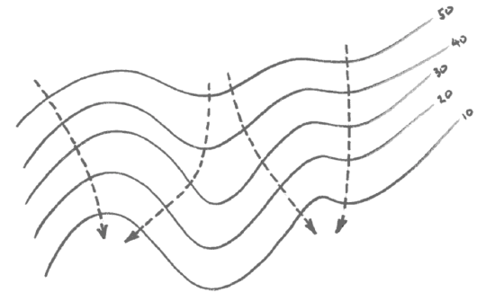
What’s going on is that the water, or you, are passing downward along what’s mathematically called the gradient: the route of steepest descent. You can trace out such routes of steepest descent, from any given point on a sloping land surface as represented on a topographic map, by drawing curves that are everywhere normal to (i.e., at right angles to) the topographic contour lines (Figure 3-46). Doing this by eye is not too difficult, once you get the knack of it.

Figure 3-46. Gradient curves down a sloping surface.

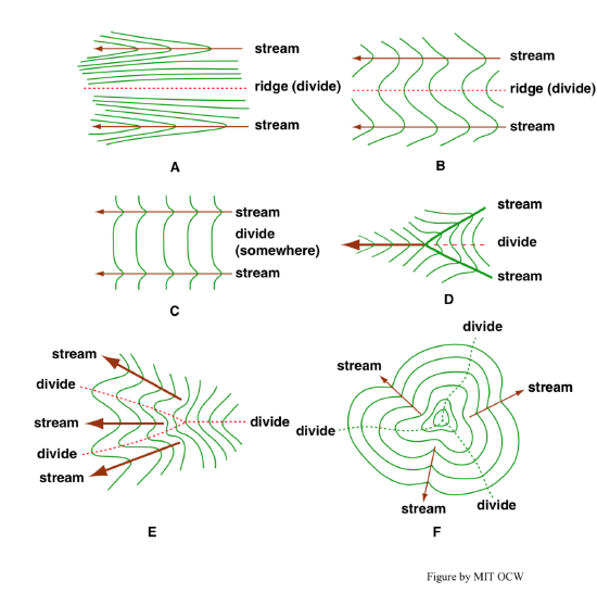
Here are some considerations on divides. When two streams are separated by a well-defined ridge crest, locating the divide is easy (Figure 3-47A). When the ridge crest itself slopes (Figure 3-47B) or is broad and not well defined (Figure 3-47C), the job is not as easy. The divide between two streams that join together at a confluence at some point ends at that confluence point (Figure 3-47D). At their high ends, divides meet can meet at the “crotch” of a Y-shaped mountain slope (Figure 3-47E) or at the summit of a hill or mountain (Figure 3-47F).

Figure 3-47. Considerations on stream divides. A) Two streams separated by a well-defined ridge crest. B) Two streams separated by a sloping ridge crest. C) Two streams separated by a broad and ill-defined ridge. D) Stream divides in the vicinity of a confluence. E) Two stream divides that merge into a single divide upslope. F) Stream divides meeting at the crest of a hill.

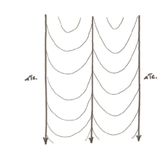
What follows is a rather lengthy “home experiment” that should be useful to you if you are having trouble dealing with the concept of stream divides. Start with several cylinders, which could be tall soda bottles with tops and bottoms cut off, or fat mailing tubes (probably the best), or the cylindrical wooden posts from an old bedstead. (Mathematically, these are circular cylinders.) Make them all the same length, ideally several times the diameter of the cylinder. Cut each through lengthwise, along a plane parallel to the axis of the cylinder but offset a bit. Keep the bigger pieces and discard the smaller. These bigger pieces should look like fireplace logs that have been split down the middle but with imperfect aim. Now place them side by side on a rigid planar surface like a cutting board, with adjacent edges touching. The result should look a little like a giant washboard. (Washboards are a disappearing item; have you ever seen one, much less use one?) Put the cutting board with its cylinders in your bathtub, with one of slowly with water, in equal increments of depth, each time stopping to mark, with a permanent-ink felt-tipped pen, the water line on the surfaces of the cylinders. You will have to solve for yourself the problem of keeping the cylinders from floating away in the process. Now drain the water and view the bathtub from a point directly above, way up near the ceiling of your bathroom. What you want to try to see is a topographic map of your tilted-cylinder model. (You might have to squint a bit to help your imagination. If you are into photography, the best thing would be to put yourself high above the model and take a telephoto shot.) The result would look something like what is shown in Figure 3-16. (Incidentally, since the intersection of a circular cylinder with a plane that cuts the cylinder at some angle less than 90° to the axis of the cylinder is an ellipse, the contours on your “map” are segments of ellipses.) The model you’ve created is not a bad approximation to many real-life examples of valley-and-spur topography.

Figure 3-48. Contour lines in your bathtub cylinder-segment model.